
Sun Path & Wind Rose
Following on from our last post on producing a master plan, this week we have a tutorial lined up for you on how to make sun paths and wind roses in Rhino 3D. We’ll be using Grasshopper and some of its plug-ins to create these representations that’ll add some flair to your analysis pages.
Note: Today’s post is directed at Windows users, as there are some features that aren’t available or optimised for Mac users on Rhino.
An important part of your site analysis is understanding the environmental conditions that will affect your proposal. Two key pieces of environmental analysis that you should include in your project are the sun path and wind patterns. These will influence decisions you make on orientation, daylighting and ventilation (just to name a few). Rhino is a great programme you can use to conduct and represent your analysis of this data.
Plugins
To make sure Rhino is set up to simulate the sun path and weather data, you need to install plug-ins for Grasshopper. Grasshopper is a plug-in for Rhino included in the software already, but you’ll also need Ladybug and Honeybee, which are plug-ins for Grasshopper.
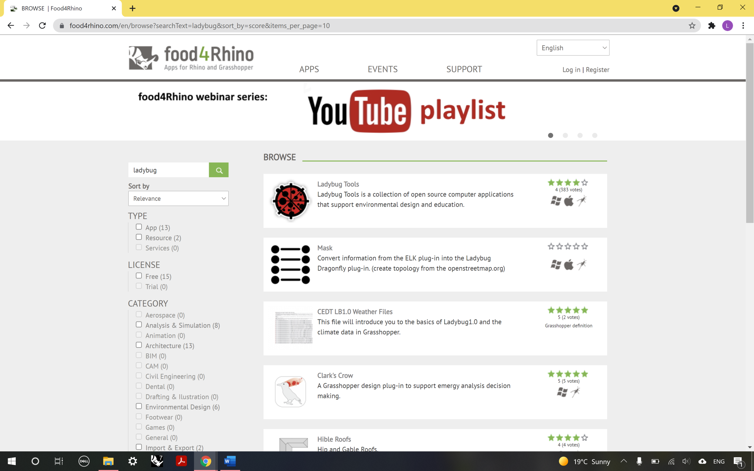


Go to food4rhino.com, the site from which you’ll be downloading the required plugins. You’ll need to make an account before you download the files you need.
Search up Ladybug, and select the Ladybug Tools options from the search results.
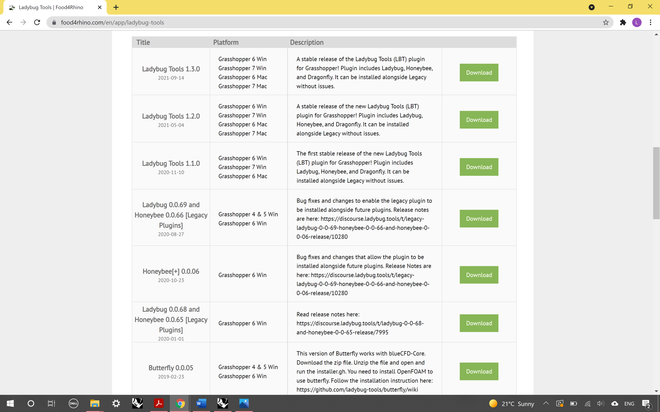
Install the Ladybug 0.0.69 and Honeybee 0.0.66 plugin. This version is what we were introduced to in our workshops at university, and I found that I ran into problems when I installed a different version of the plug-in to what we were being shown.
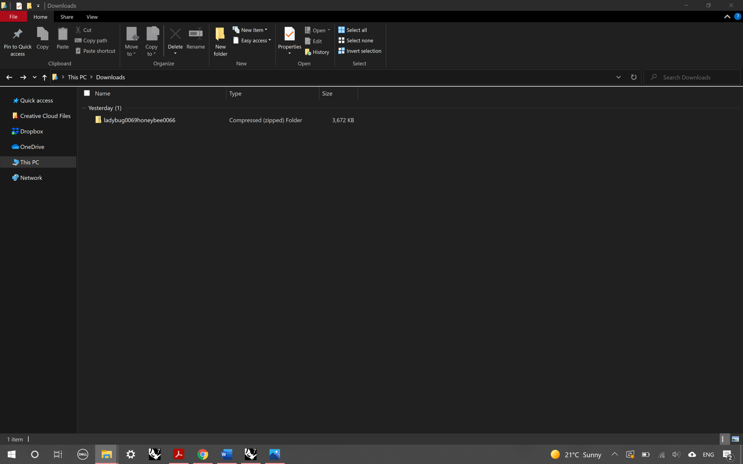
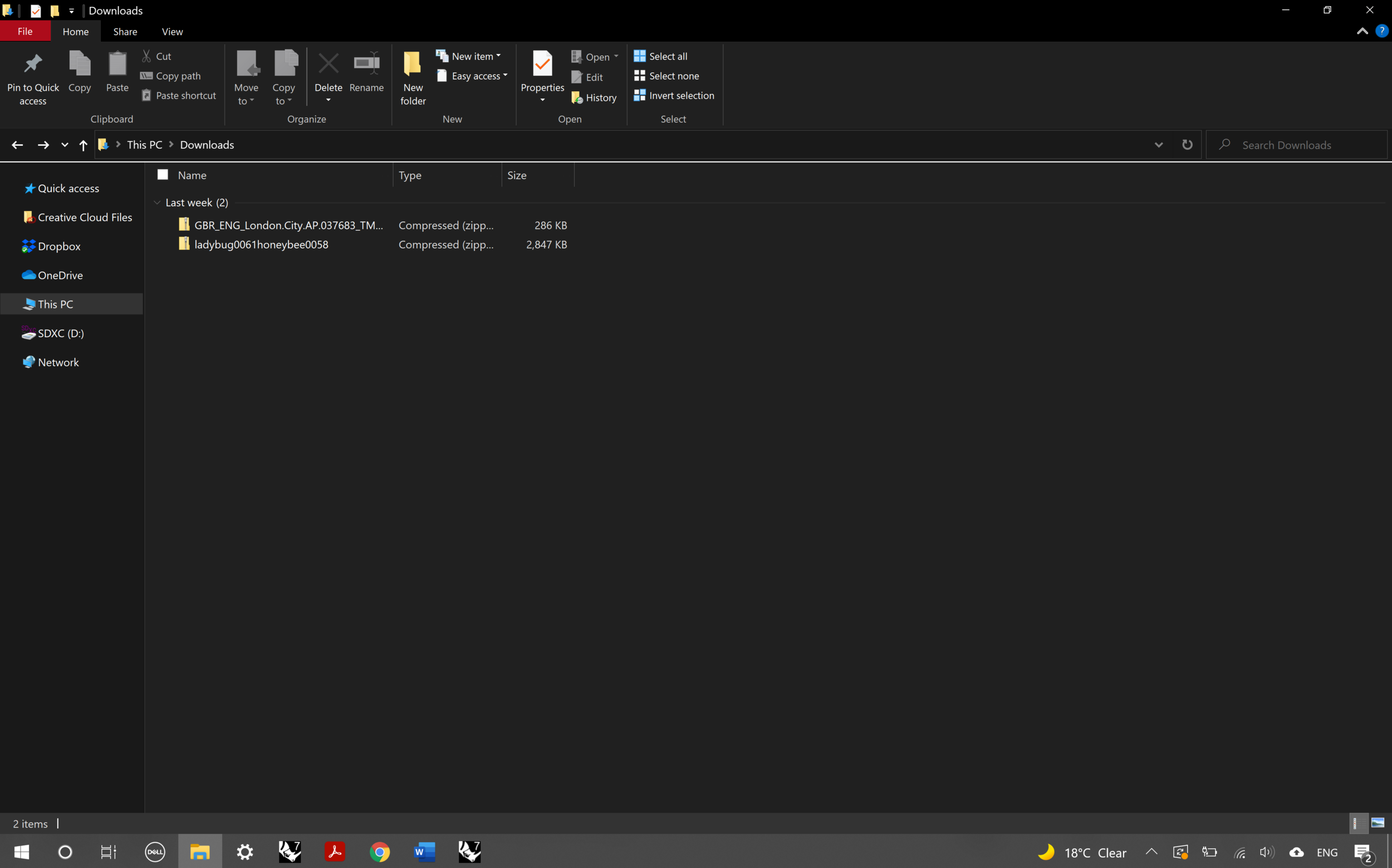
You should now have the plugins in your downloads folder in a ZIP File. Next, we’re going to extract the files into the user object folder.
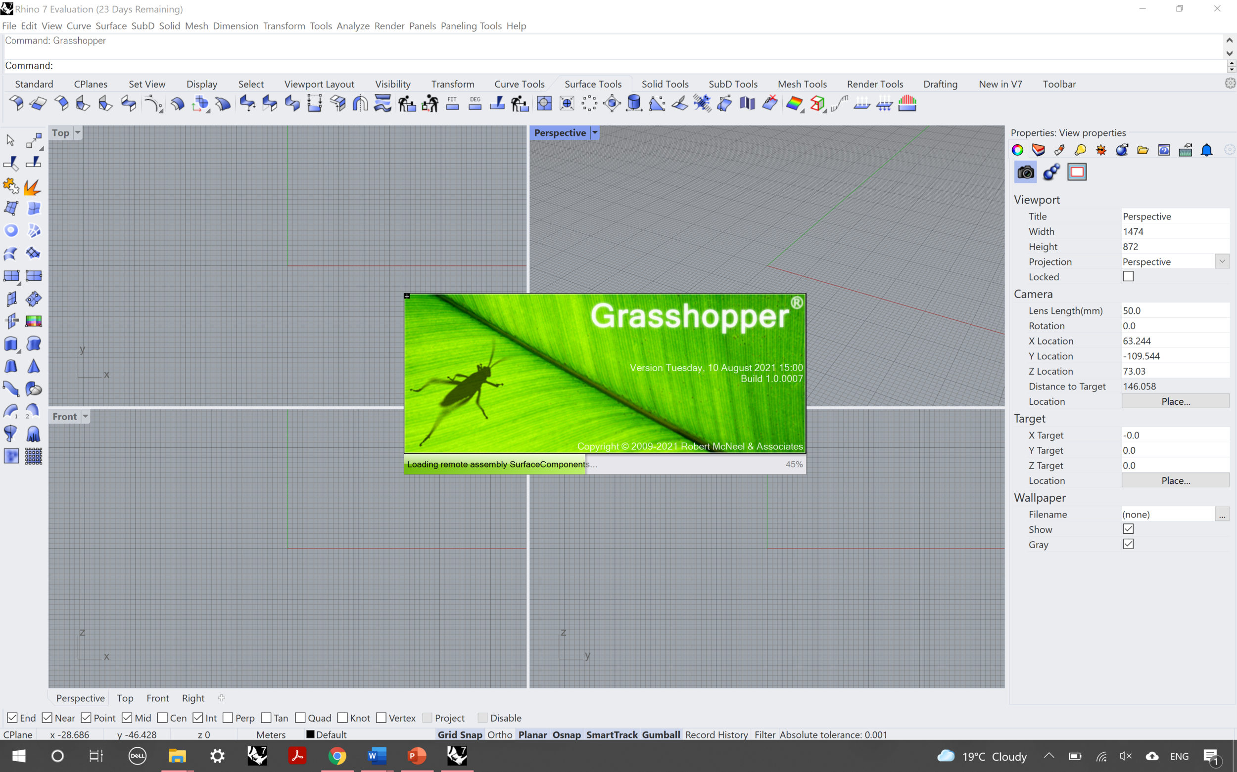


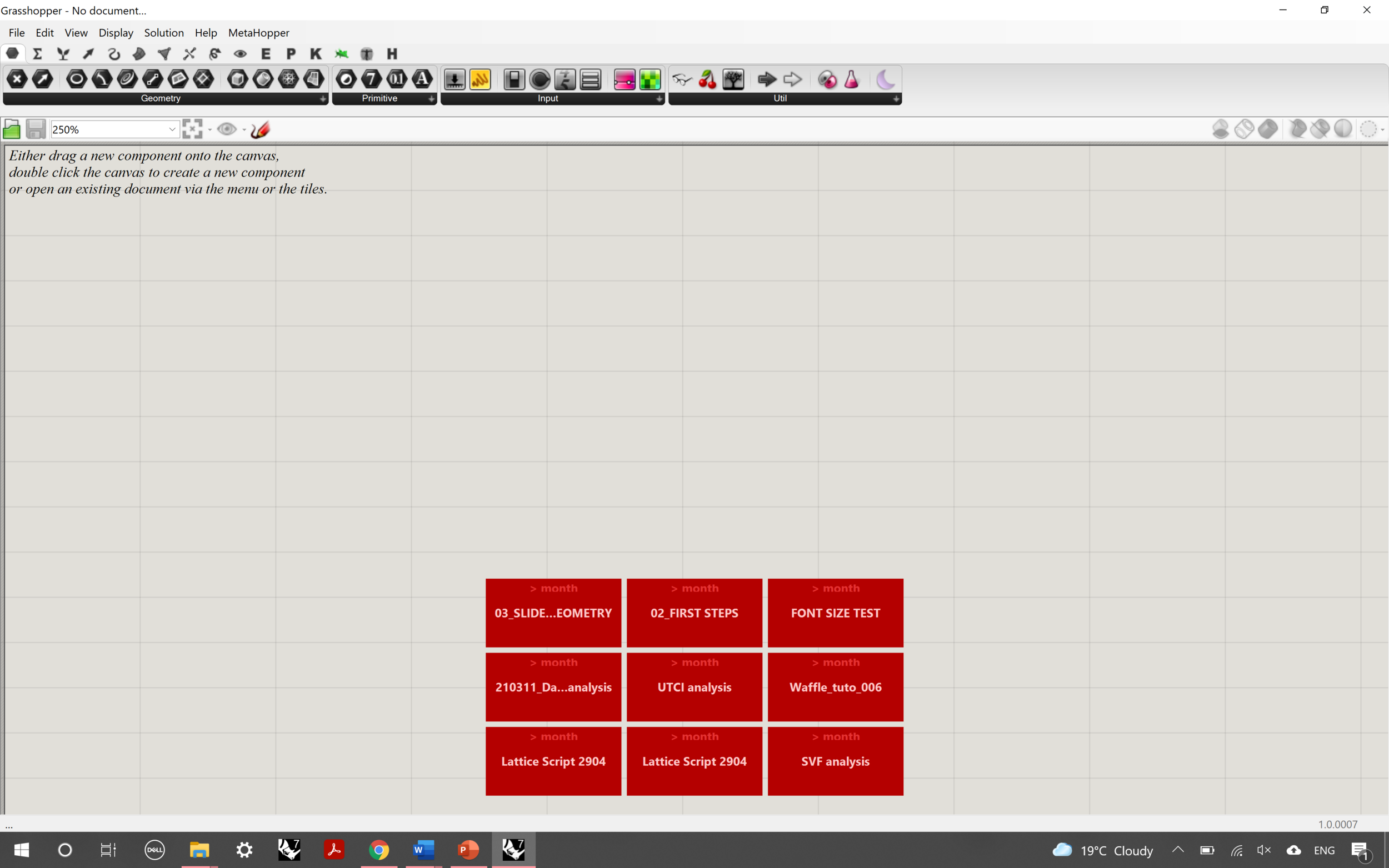

Open a ‘Large objects’ Rhino template (in mm) and load Grasshopper in the commands or menu bar.
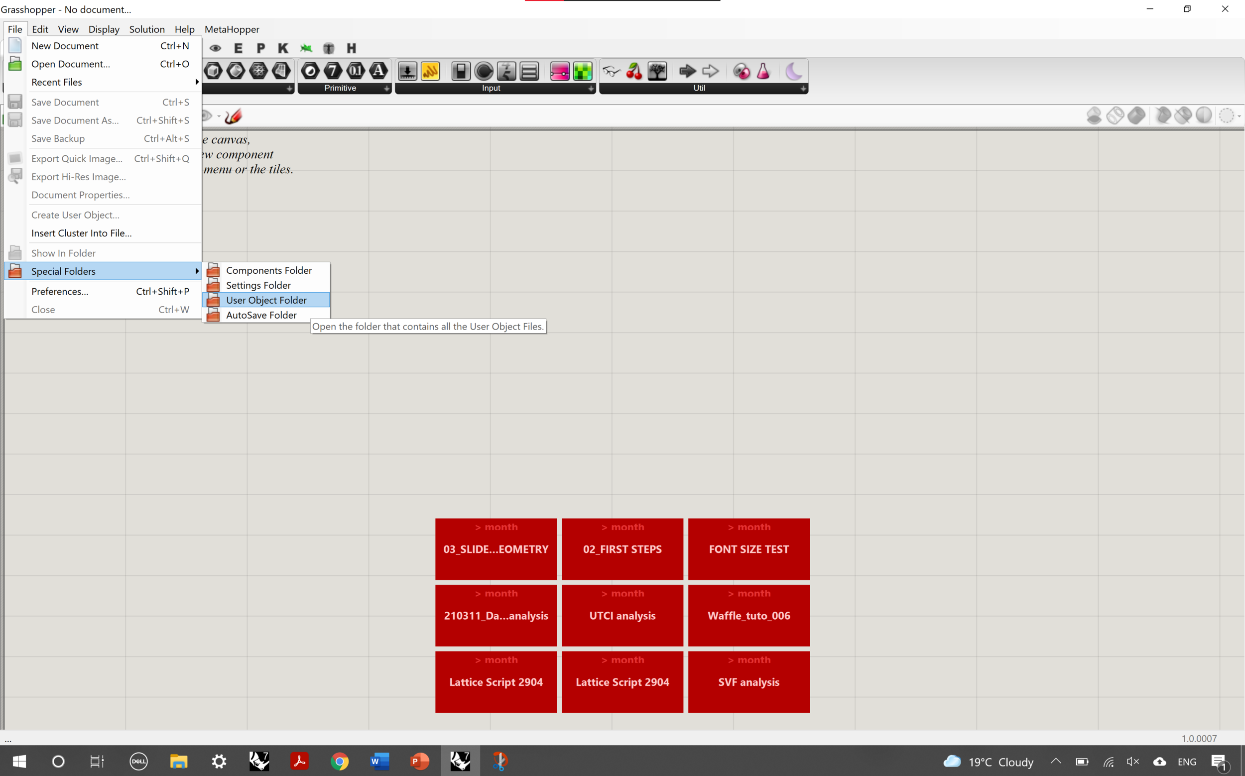
Go to File – Special Folders – User Object Folders. This should open up a new window, where you’ll be transferring the plugin files to.
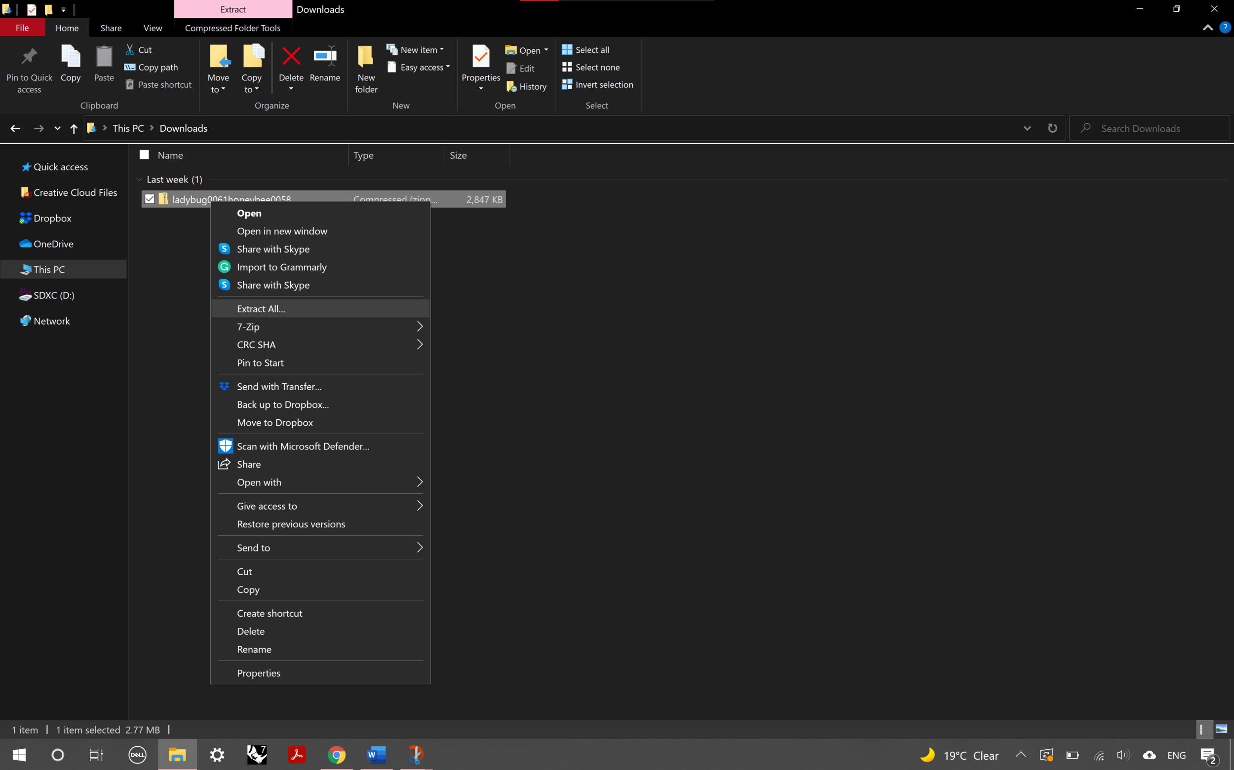

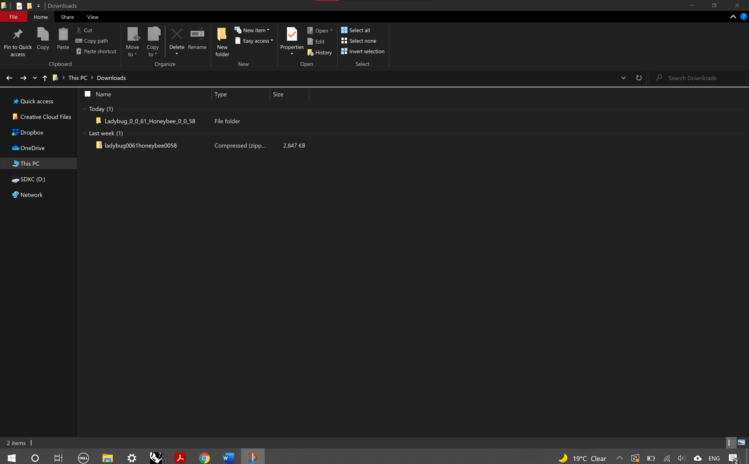

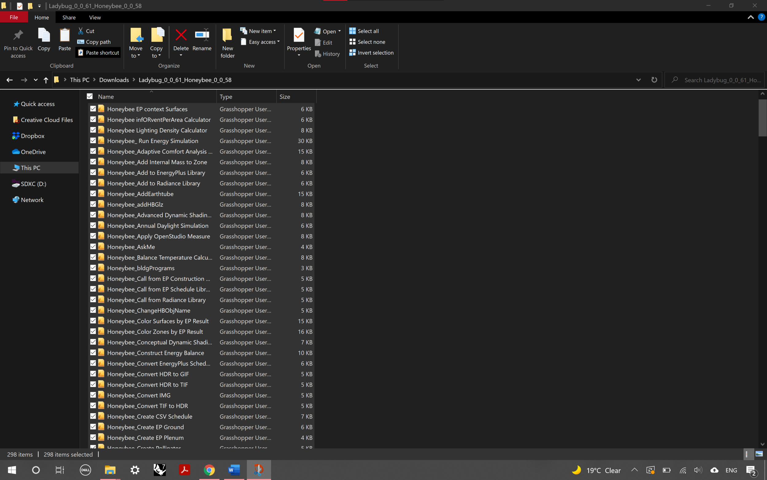

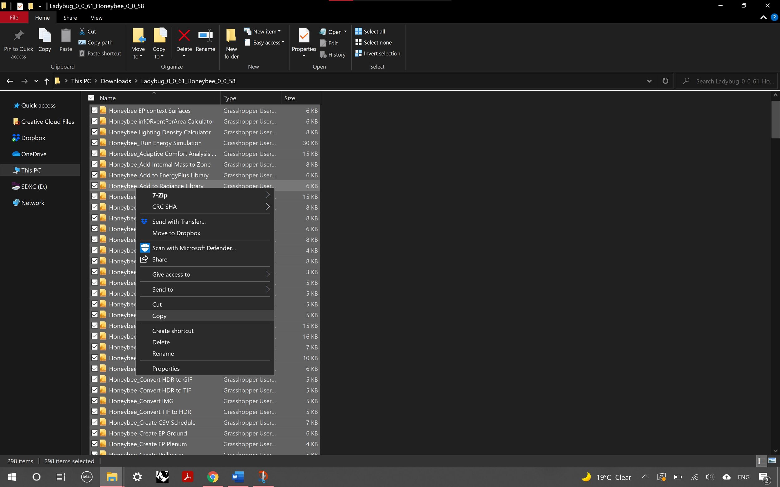


Extract the files in the ZIP folder you downloaded (I extracted mine back into the downloads folder).
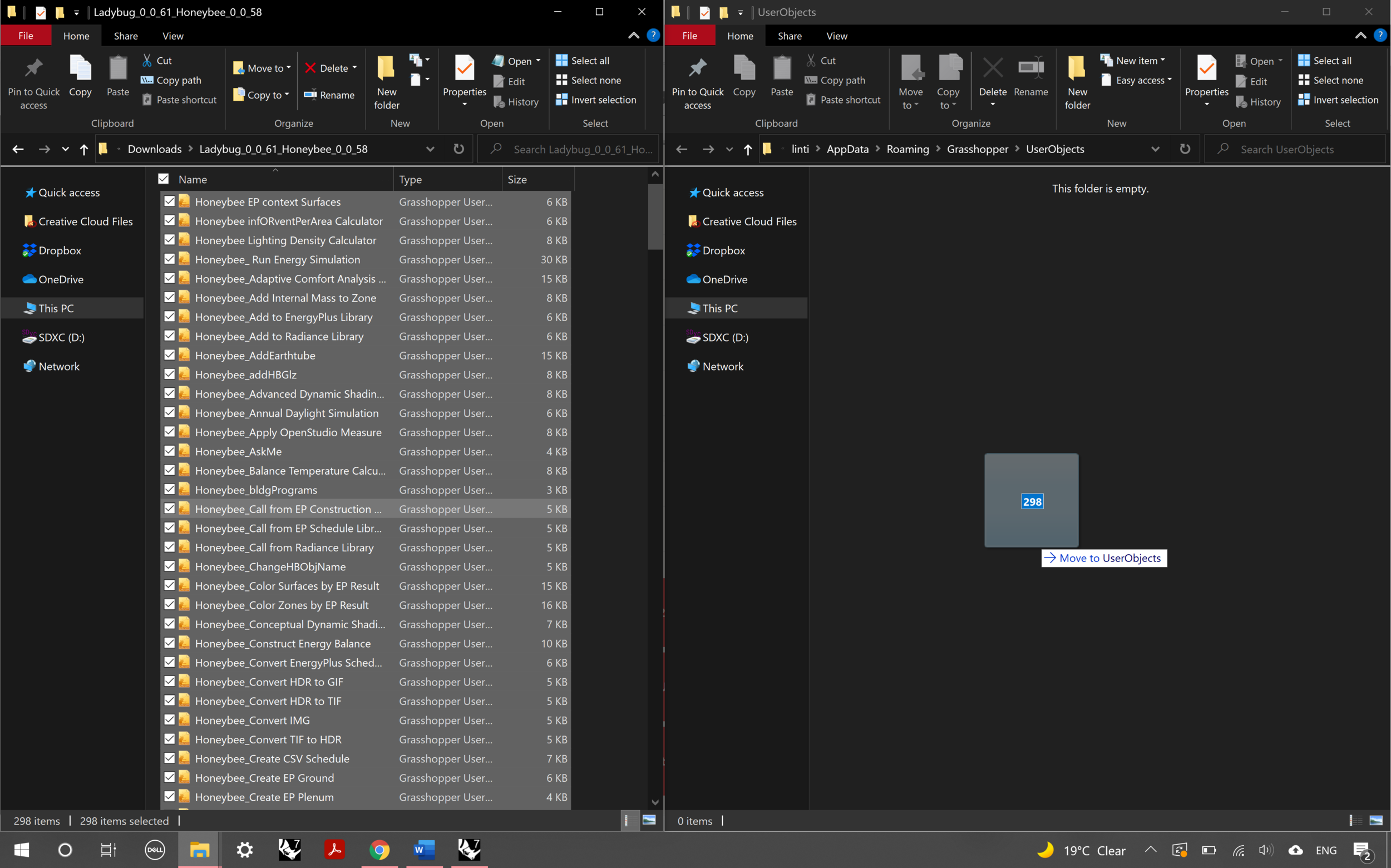
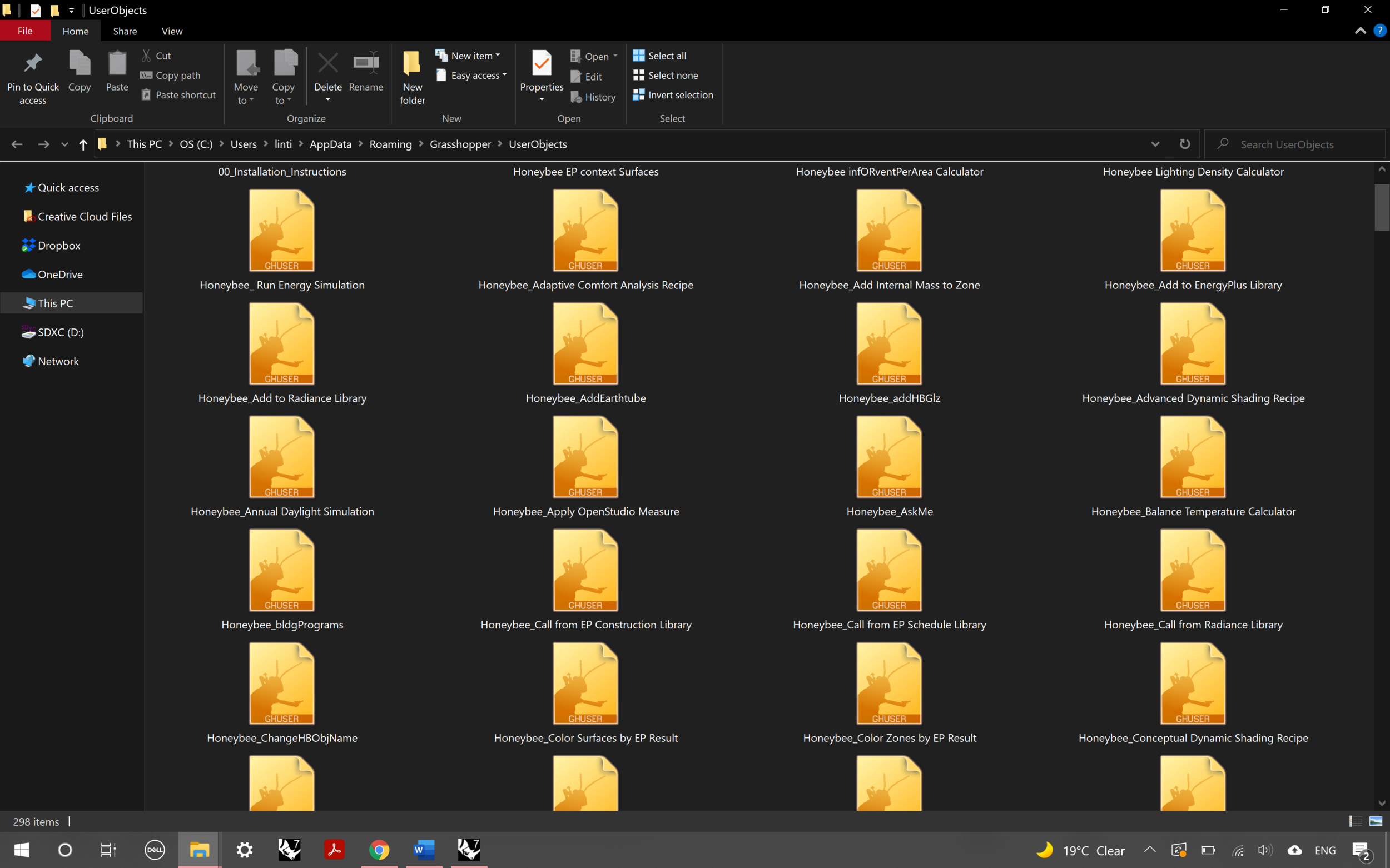
Drag the files from your downloads folder into the User Objects Folder, as demonstrated in the split-screen photo above (slide 5).


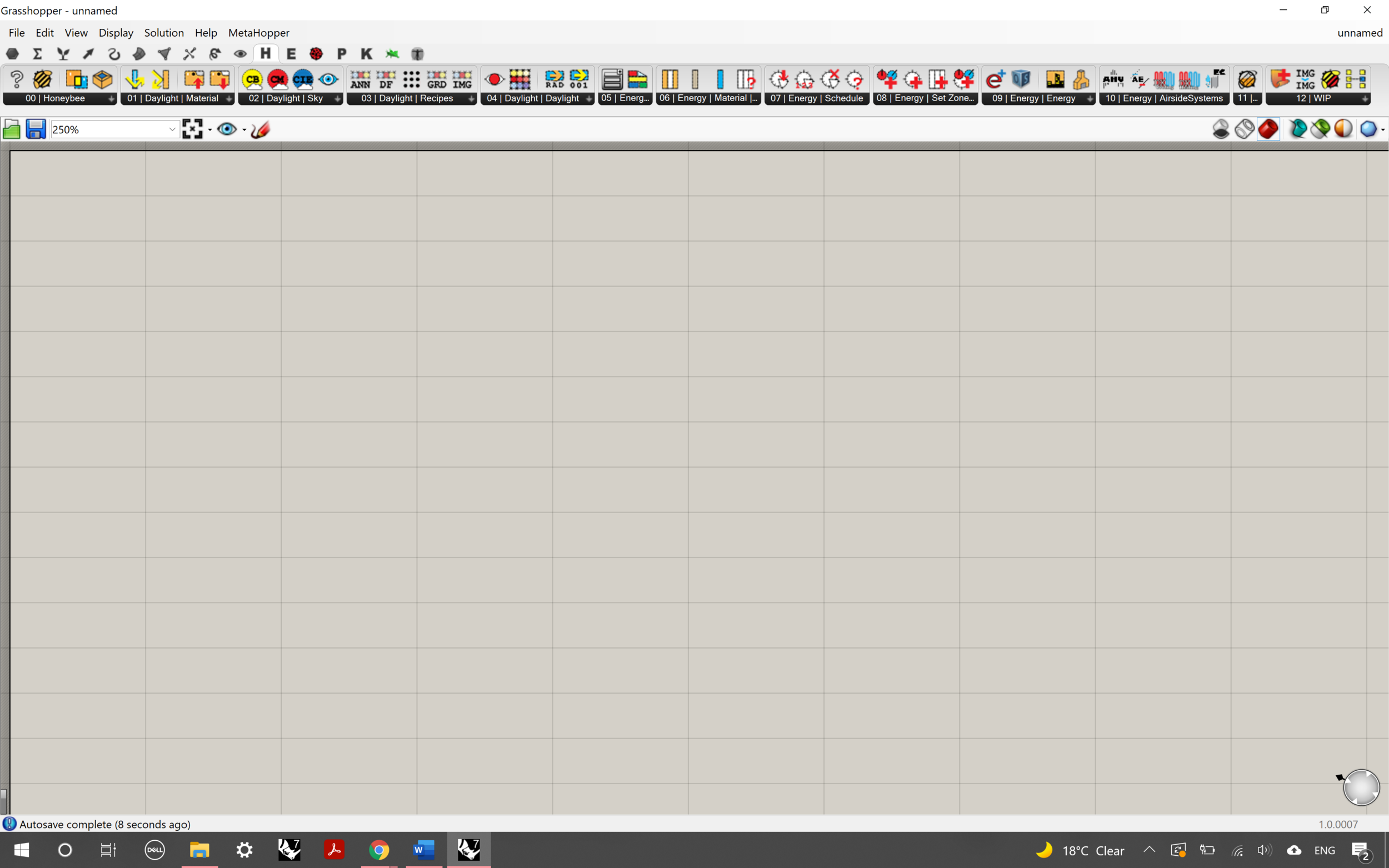
Restart Rhino and open up an empty Grasshopper File. You should see the plug-ins added in at the top in the menu bar.
EPW Weather Data Files
Although the actual sun paths and wind roses are created on Rhino, you’ll need to source the weather data to inform the scripts externally.

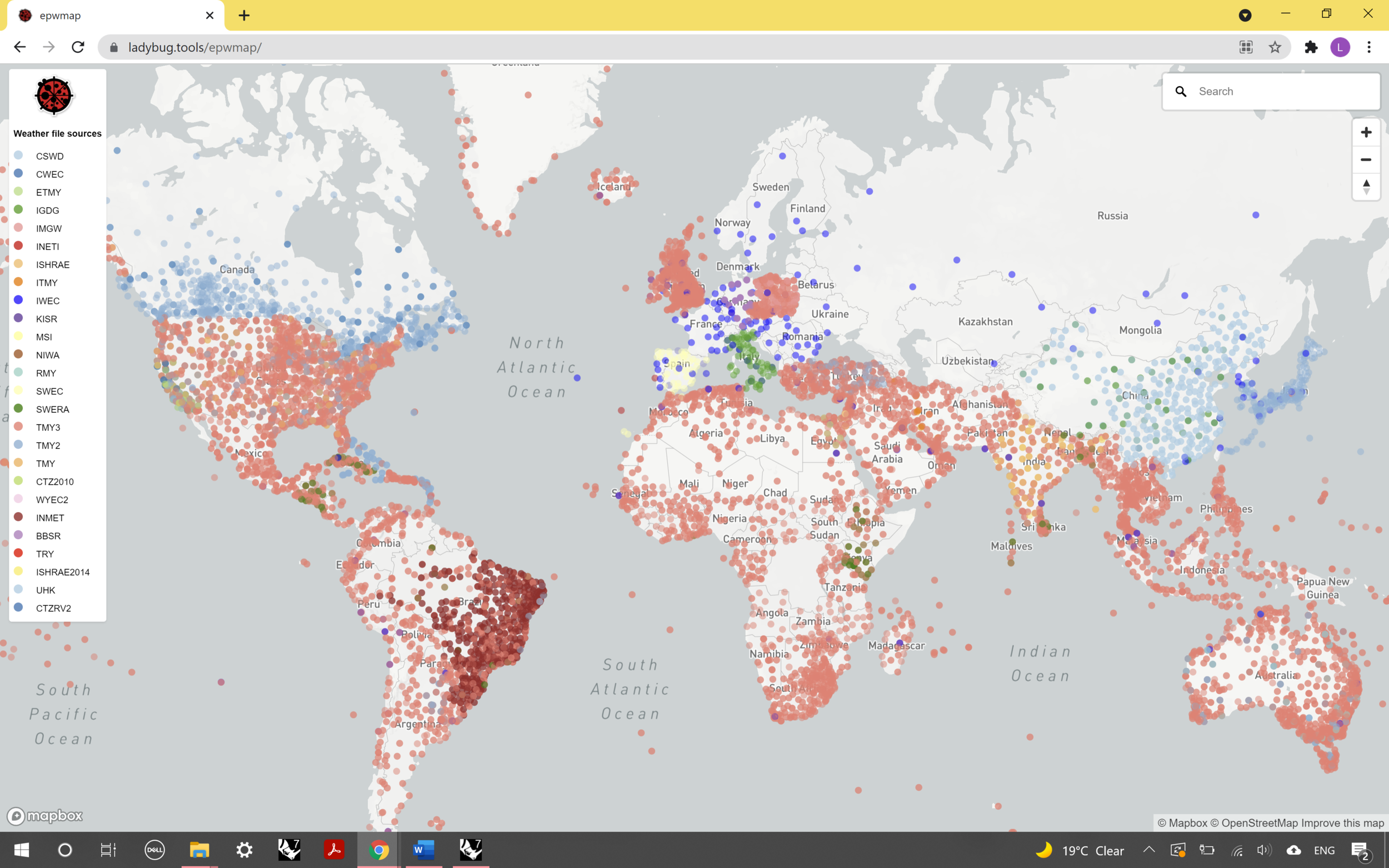


Go to epwmap (a part of the ladybug.tools website). A dotted map will appear demonstrating the locations for which some sort of weather data is available.
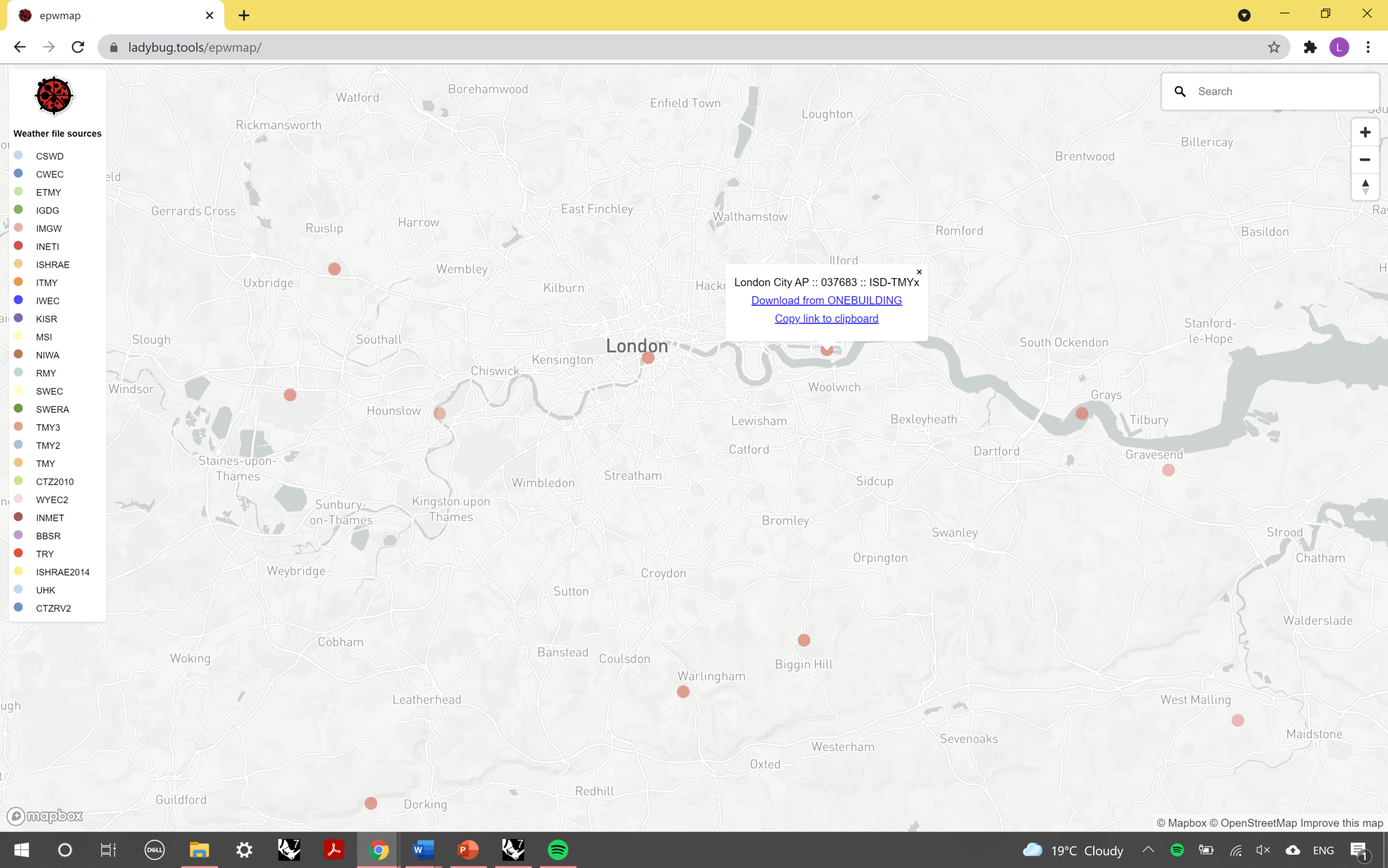
Find and select the file closest to the location your site is in. Bear in mind that the data is there to give you an indication of the environmental properties in regards to the sunlight and wind patterns. The stations at which the measurements are taken are unlikely to be exactly where your site is, so take this into account during your site analysis if you’re using a combination of analogue testing and digital simulations.
Copy and paste the URL into your browser or click on the direct download link to retrieve the file onto your computer.
Scripts
In order to simulate and represent the weather data as a sun path and wind rose, we’ll be creating scripts for Grasshopper to run, which will entail combining components inserted into the workspace and inputting different values to amend the data we want to represent.
Sun Path


Step 1:
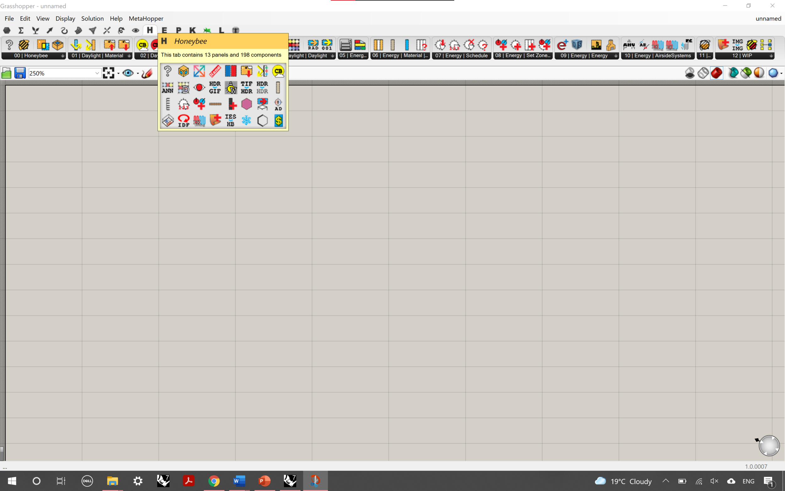
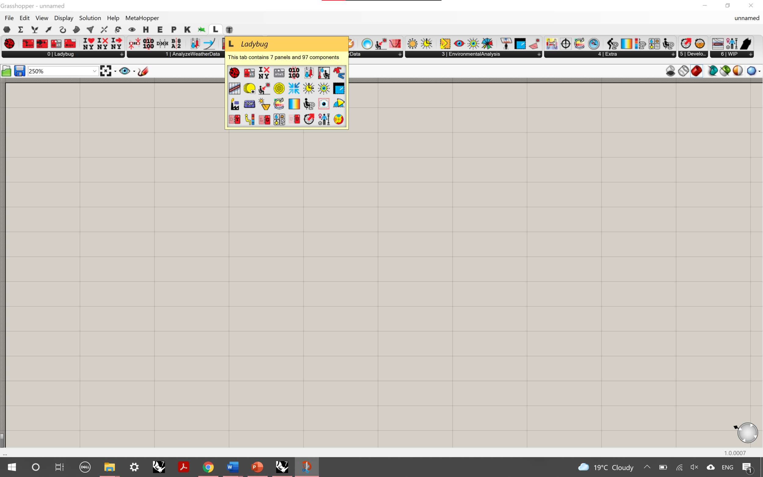
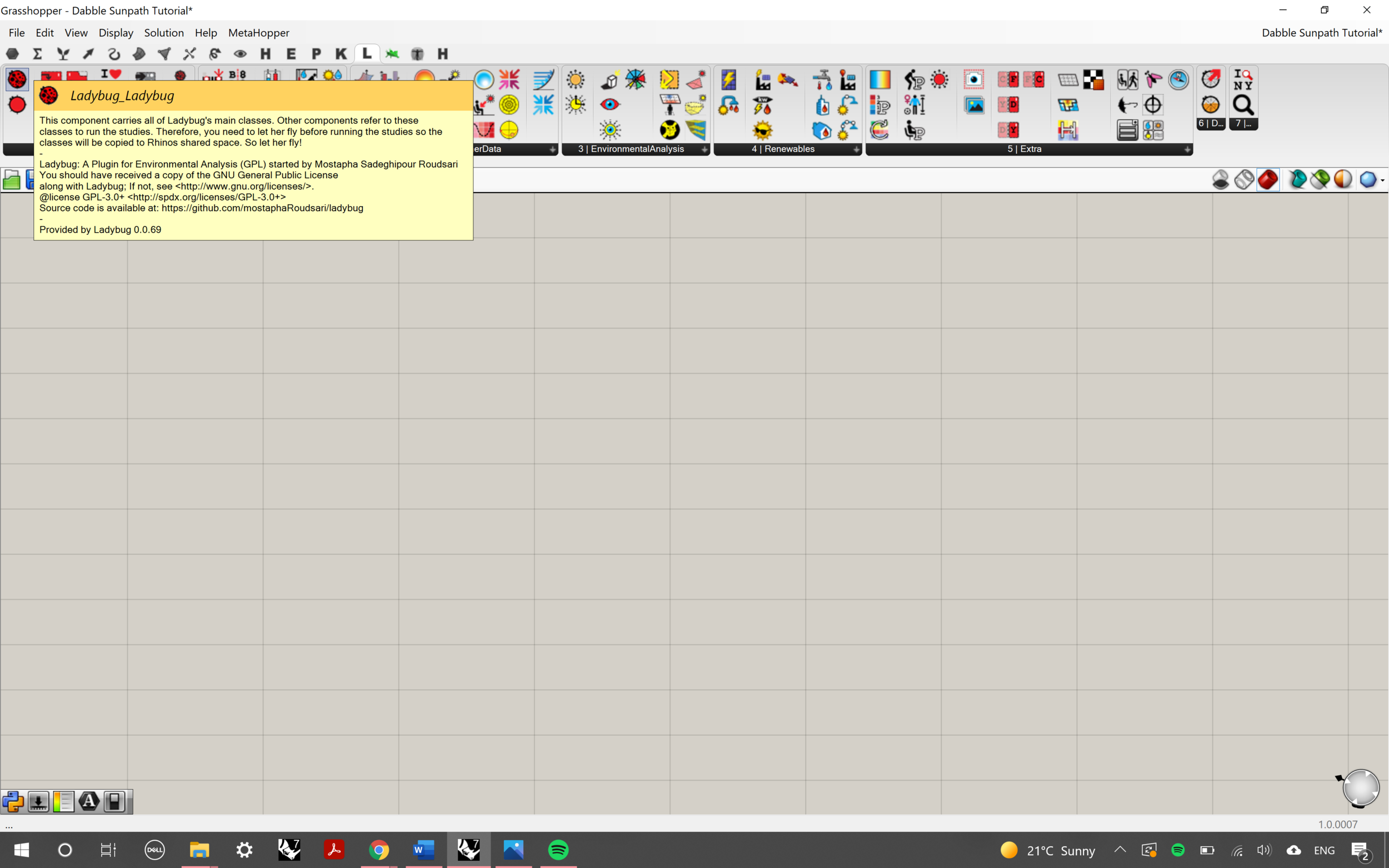
Open up a new Grasshopper file and go to the Ladybug panel, symbolised as an ‘L’ or a ladybug icon in the panels above the gridded area.
Drag the ‘Ladybug_Ladybug’ component into the workspace and place it in the top-left corner. This is one way to add components to build up your script.
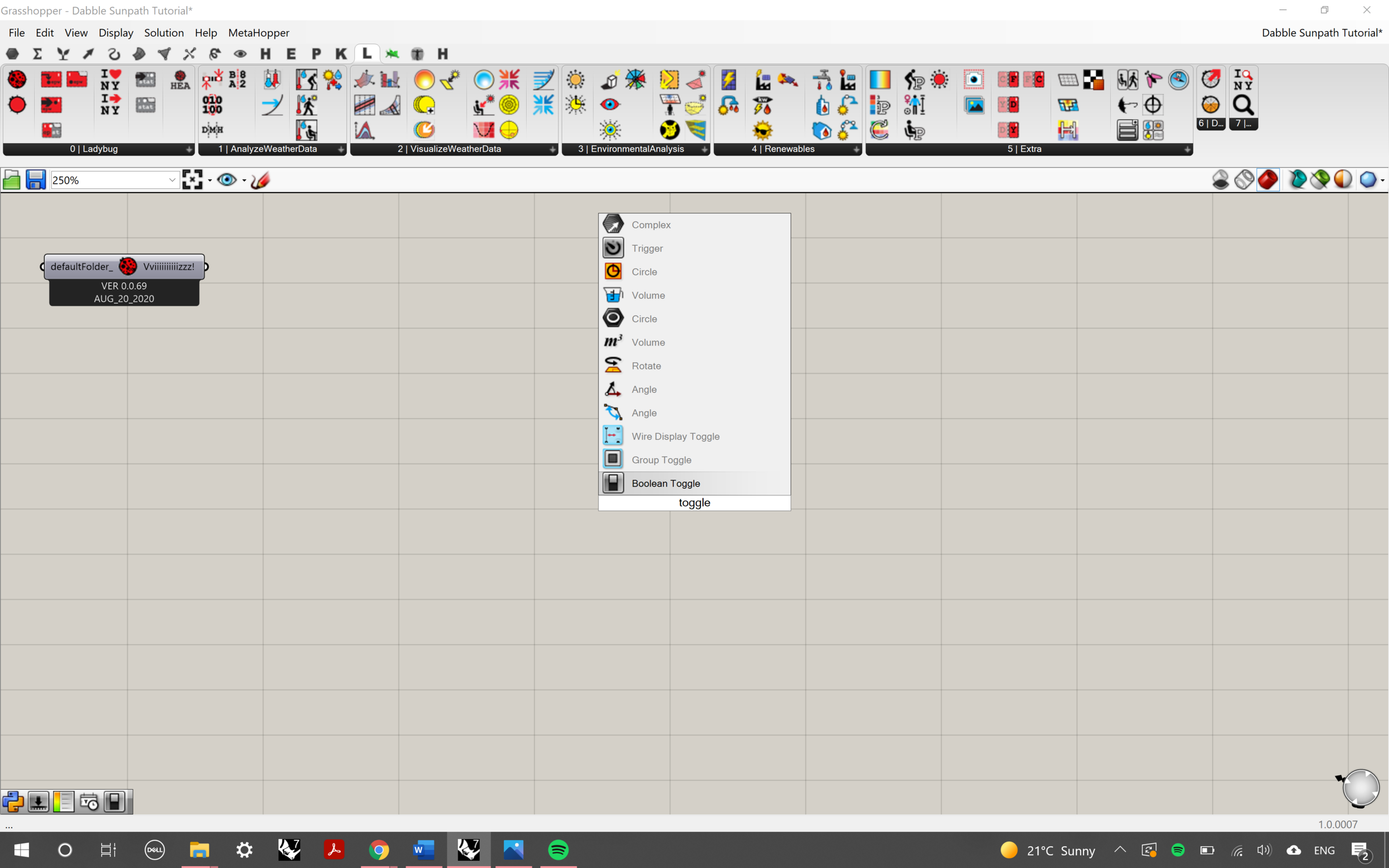
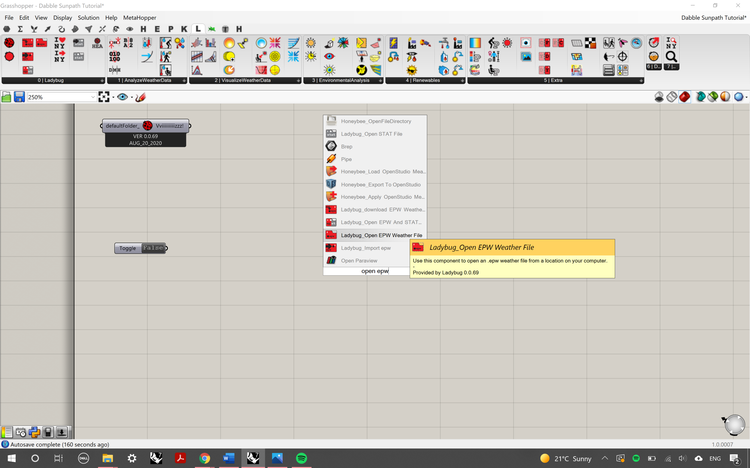
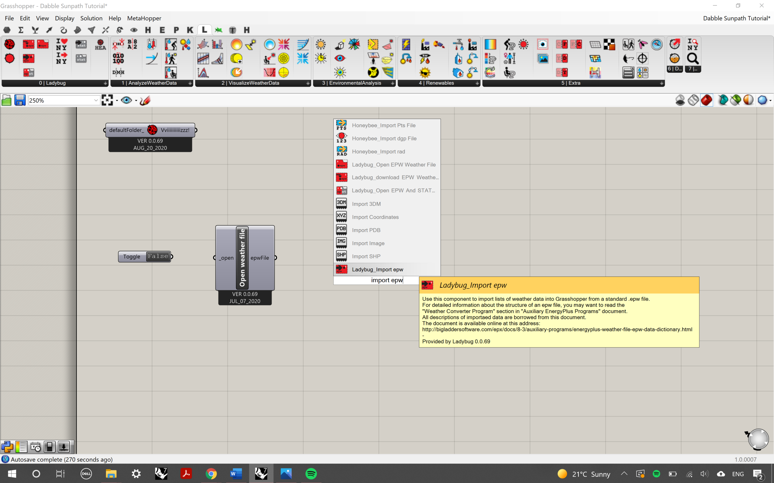
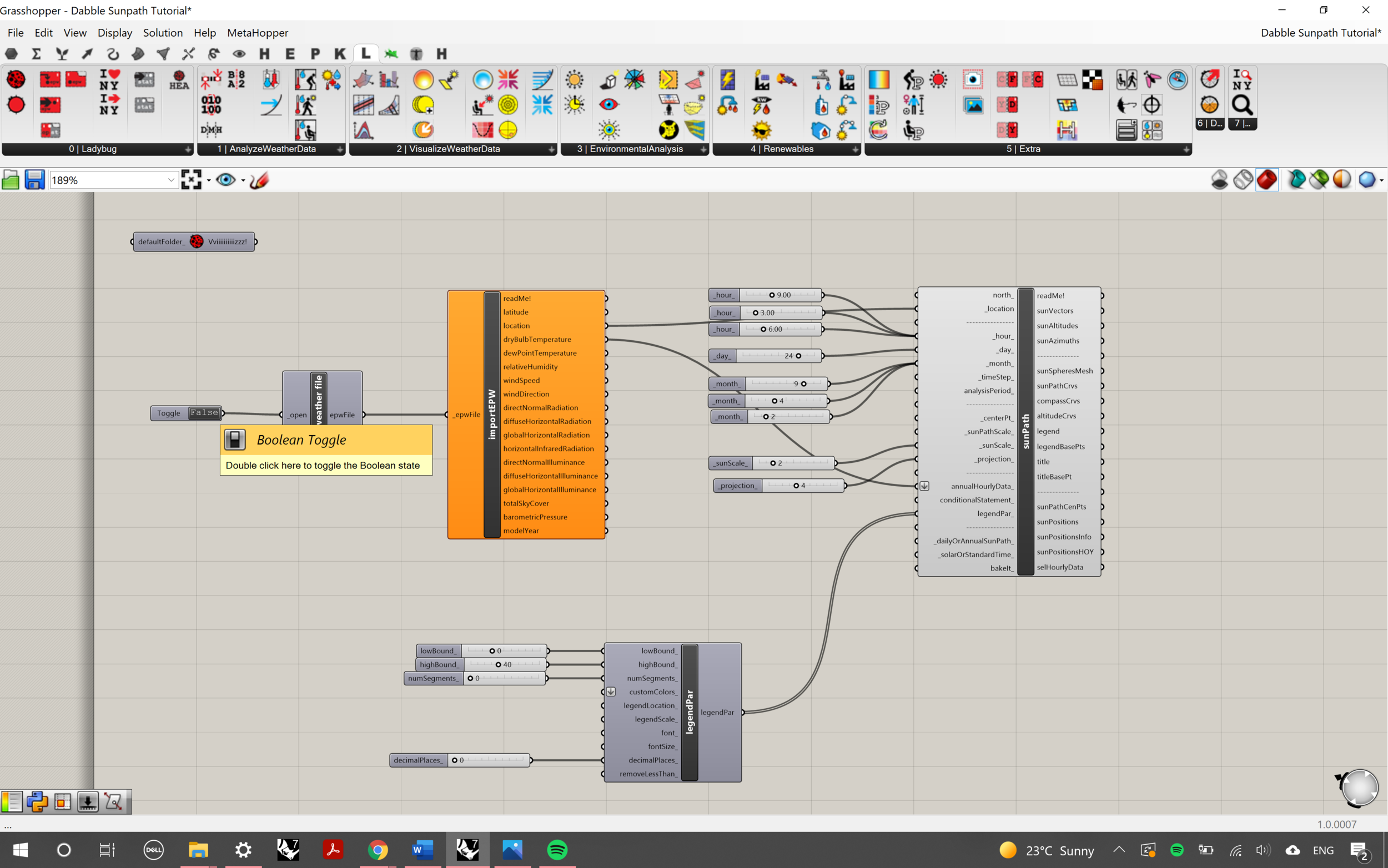
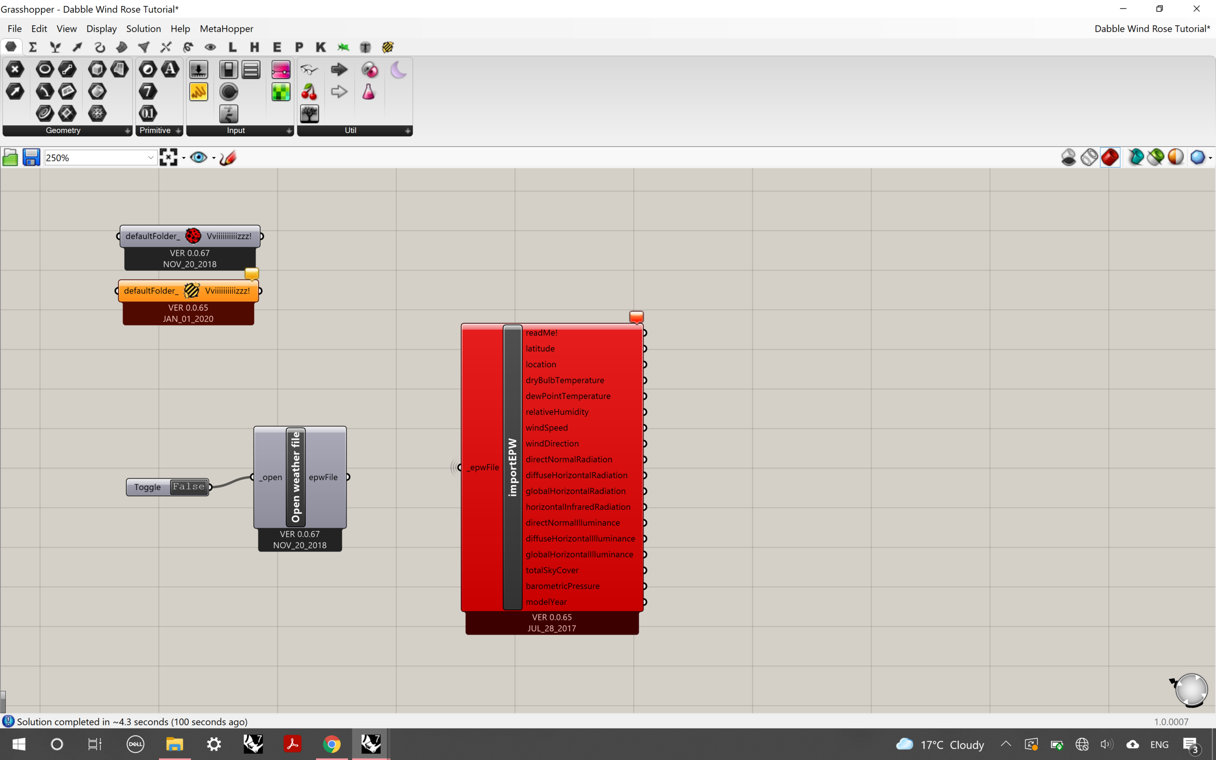
The next way is by pressing the space key (the same way you would to start up a Rhino command) to bring up the search bar. Type in ‘Toggle’ and select ‘Boolean Toggle’. Repeat this process, searching up ‘Open EPW’ and ‘Import EPW’ to obtain the next two components.
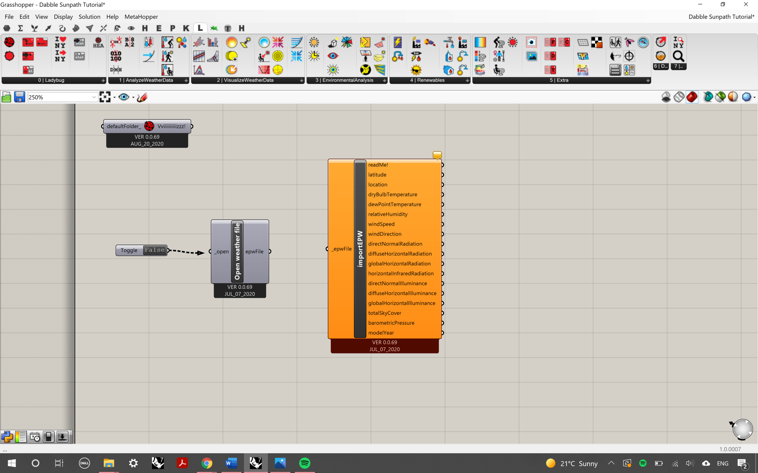
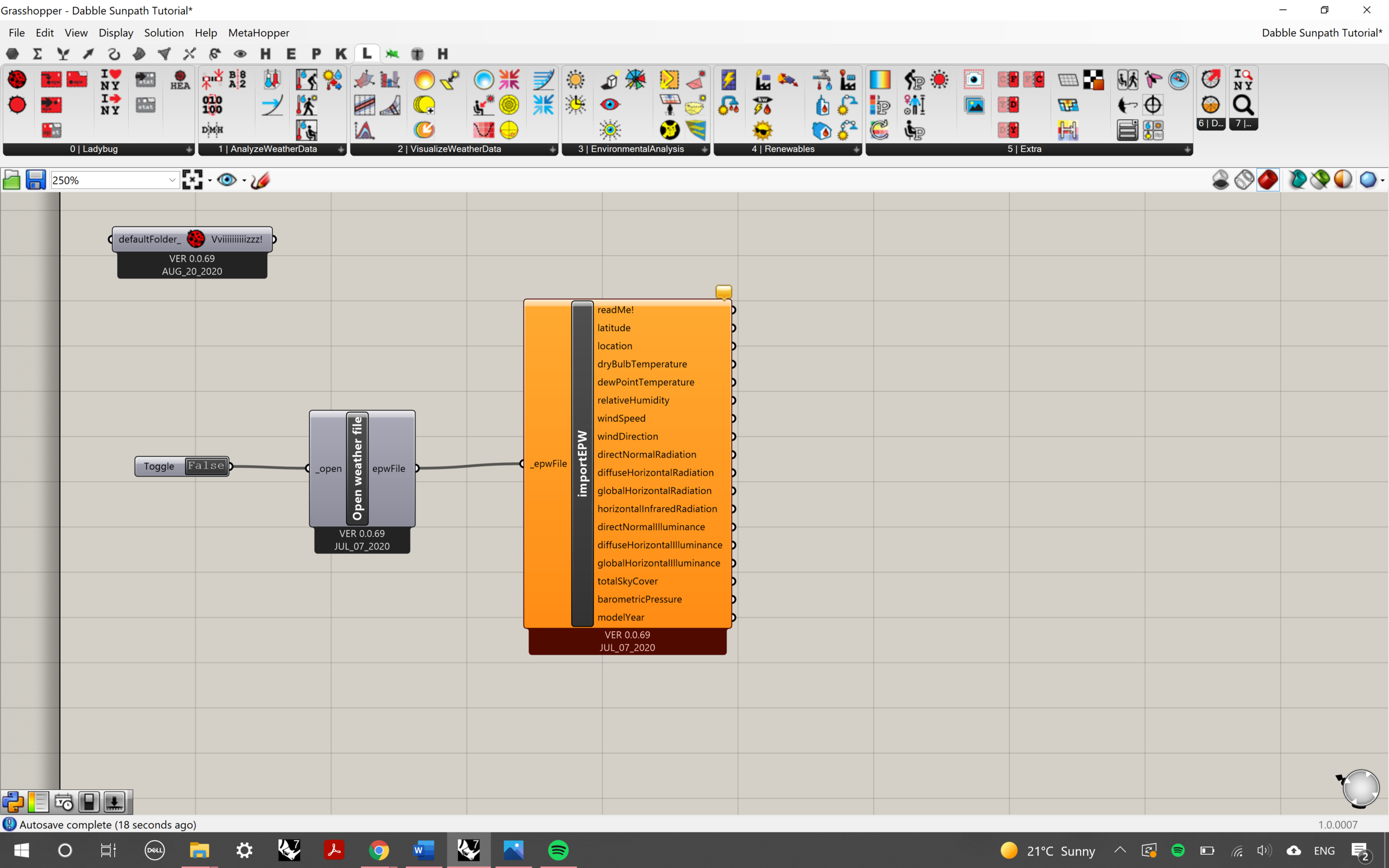
Connect the components by clicking and dragging from the white circles on the edge of the components in the order as shown in the screenshots above.
This part of the script will open up an EPW file from your computer and import the data into Grasshopper.


Step 2:
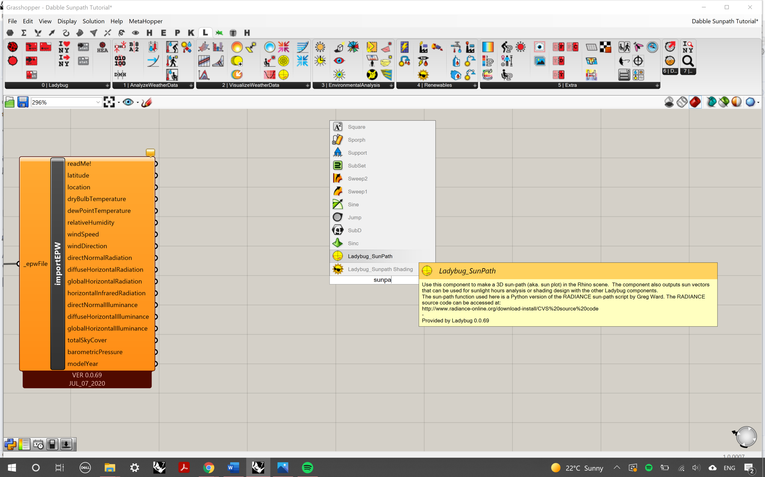
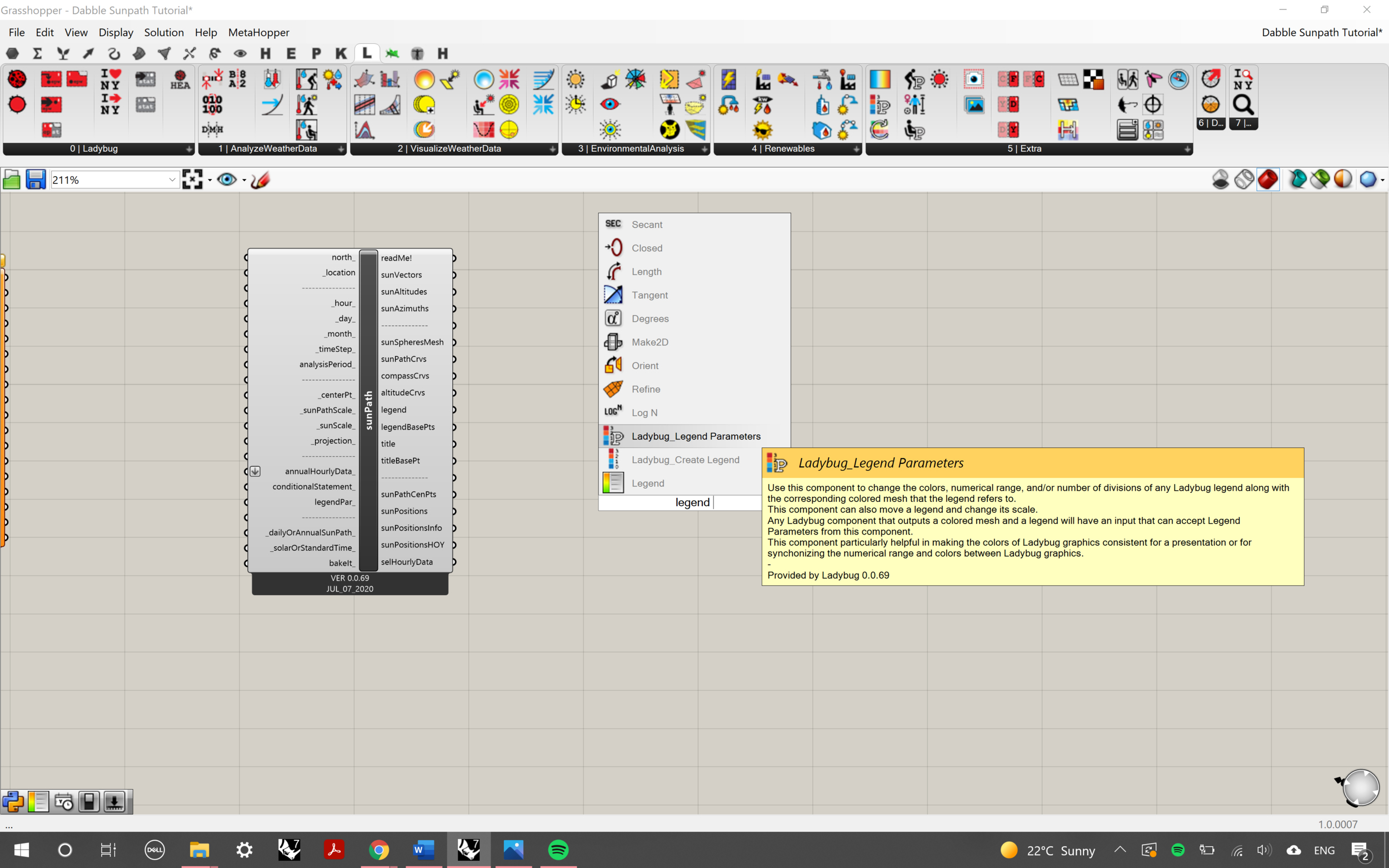
Next, we’re going to insert the ‘Ladybug Sun Path’ and ‘Legend Parameters’ components which will allow us to represent the sun’s locations and the key to go alongside the sun path.
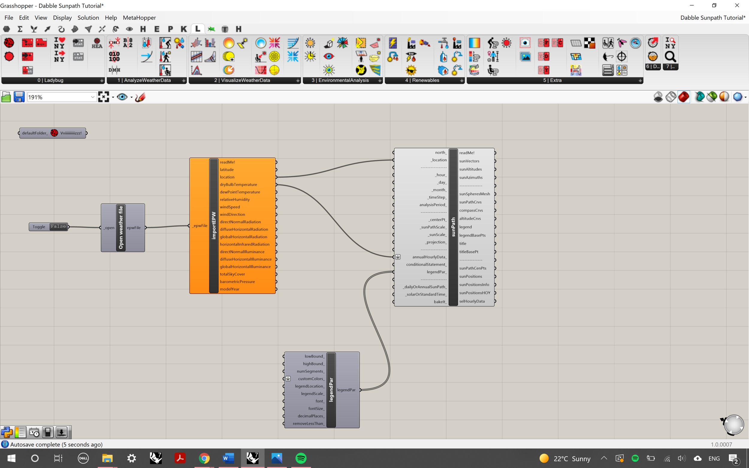
Insert the components as shown above. As you can see, there are a lot more connections on these larger components than the previous ones. You’ll need to connect the following:
location (importEPW) -> location (sunPath)
dryBulbTemperature (importEPW) -> annualHourlyData (sunPath)
legendPar (legendPar) -> legendPar (sunPath)


Step 3:
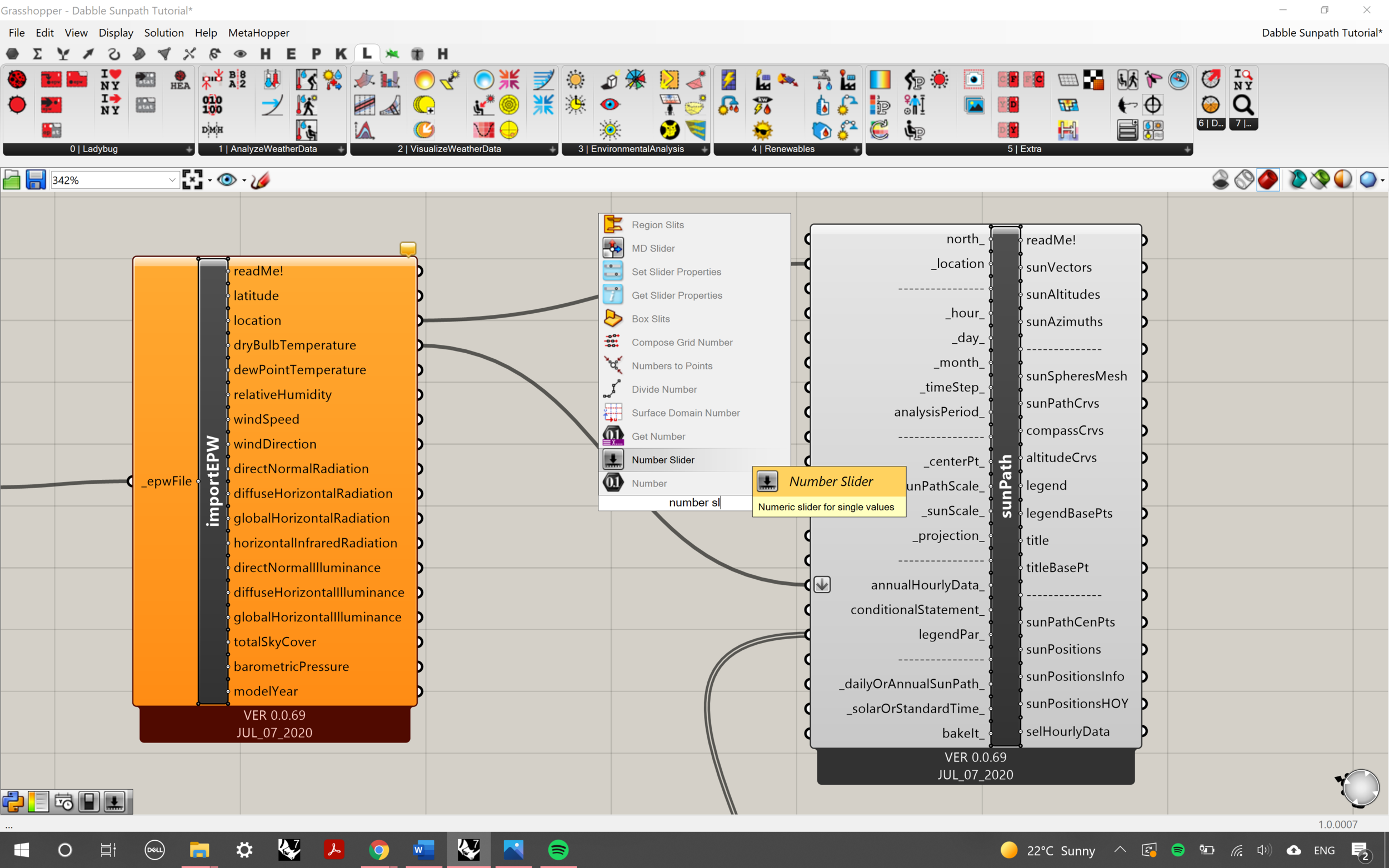
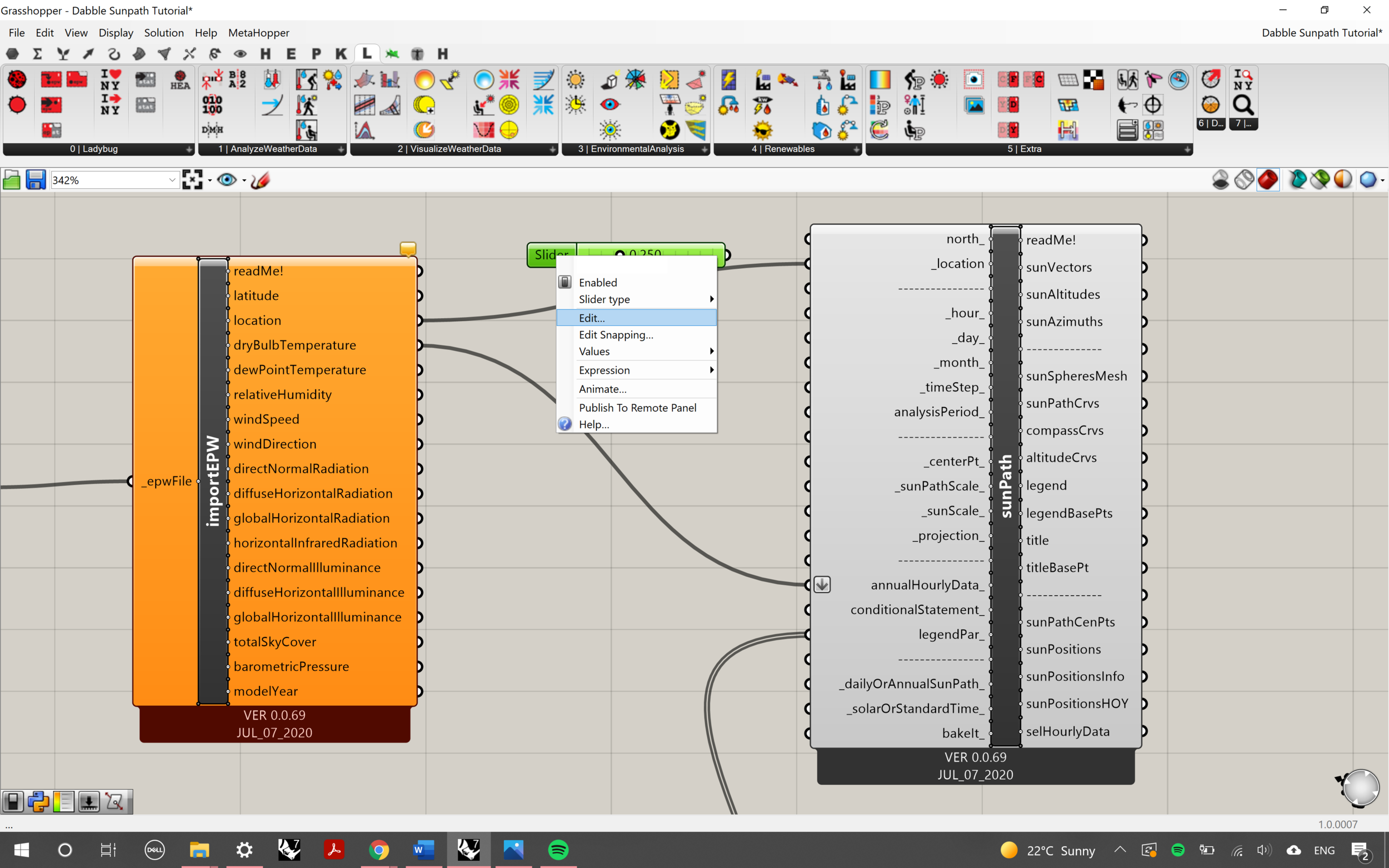
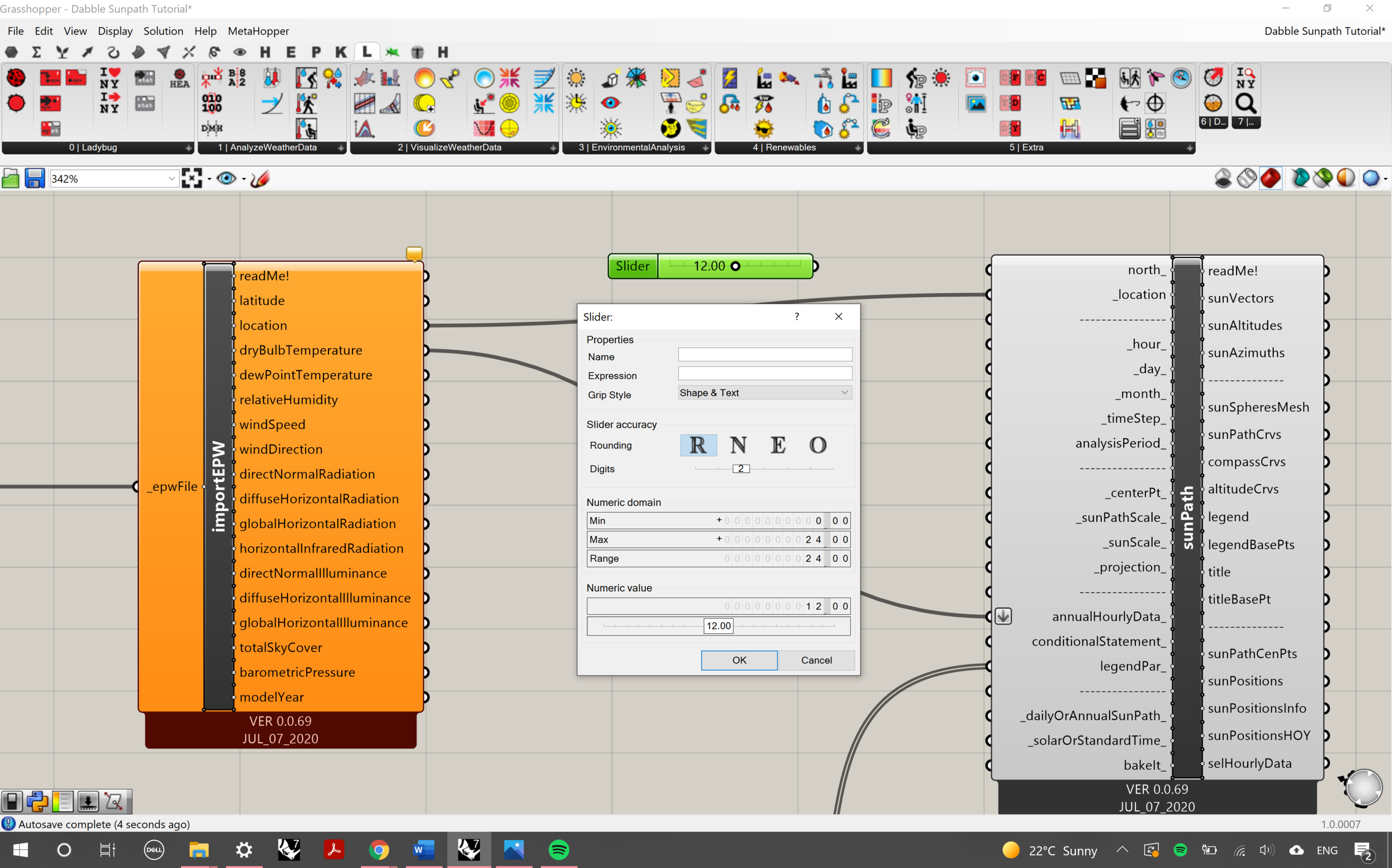
We’re going to add in some number sliders to input some extra data to toggle for the sun path representation. Press space and obtain the ‘Number Slider’ component. Right click on it and click ‘Edit’ to change the slider properties. We’ll be creating sliders for hours, days, and months, so set the properties for the sliders as follows:
Hour Slider:
Decimal Points: 2
Min: 0
Max: 24
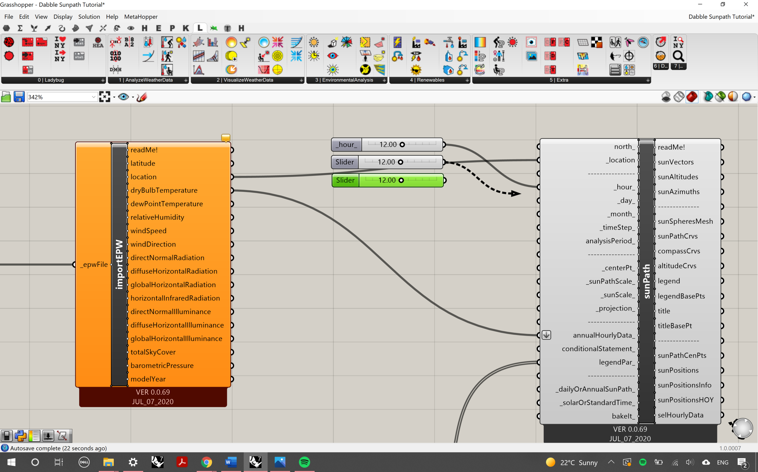
Copy and paste this twice more so you have a total of 3.
Day Slider:
Decimal Points: 0
Min: 0
Max: 31
Month Slider:
Decimal Points: 0
Min: 0
Max: 12
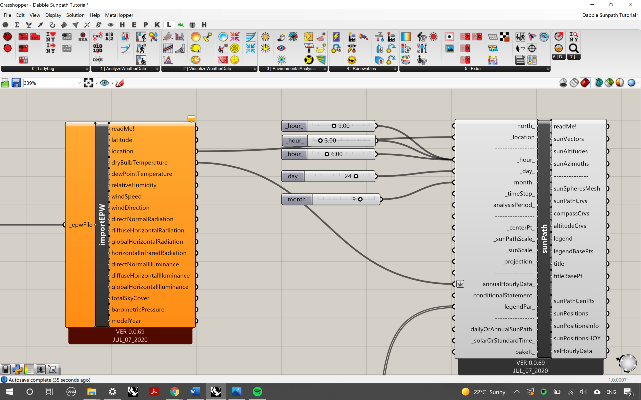
Connect the first three sliders to the hour row, the fourth to the day row and the last three sliders to the month row. Make sure to hold shift when connecting multiple sliders to one row so that the others don’t disconnect.
You should also notice that the names automatically change to the corresponding row once connected.
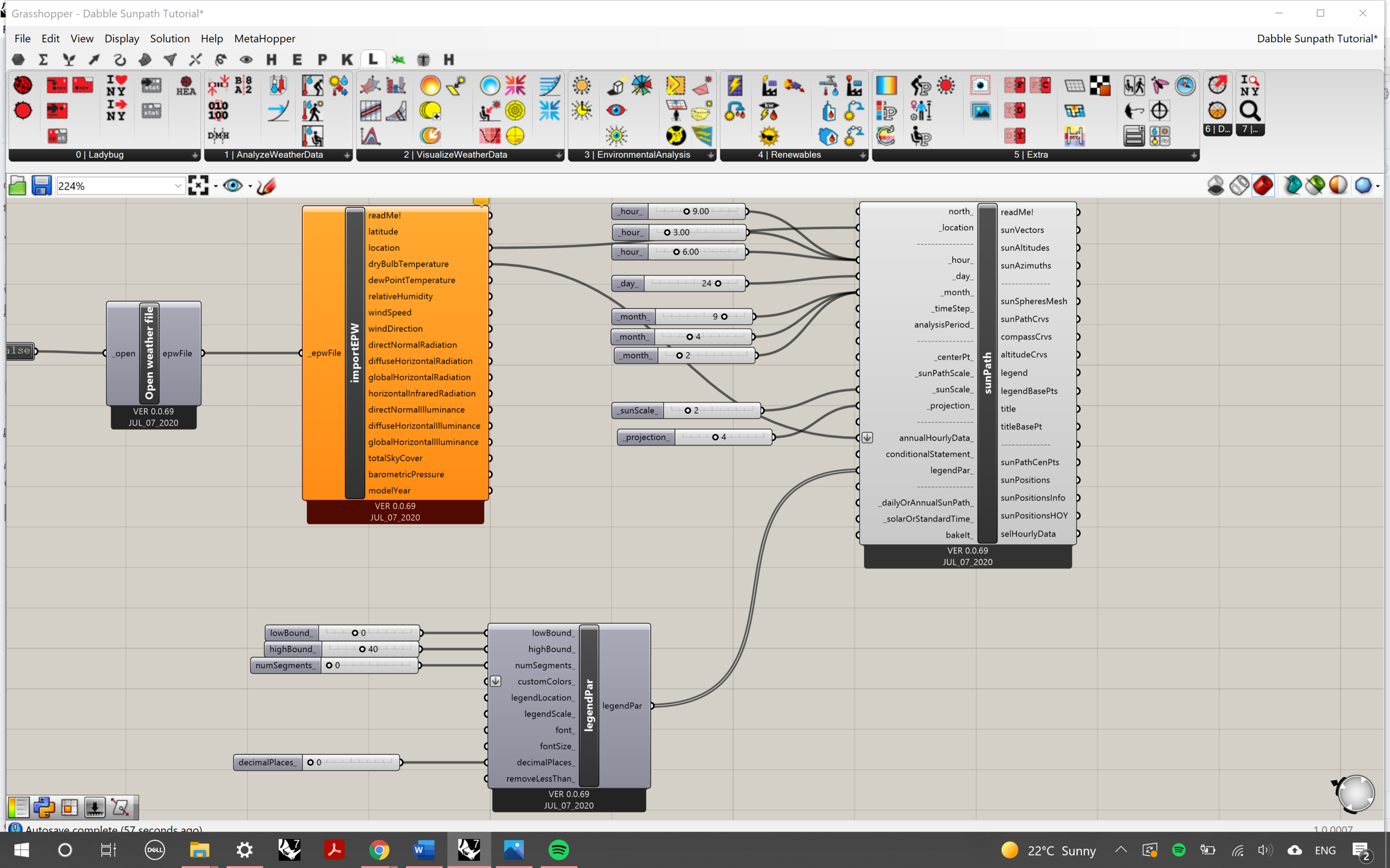
Repeat the process for the following extra sliders i.e. connecting them to the corresponding rows of the components:
Sun Scale, Projection Sliders -> sunPath input
Low Bound, High Bound, Number of Segments, Decimal Places Sliders -> legendPar input


Step 4:
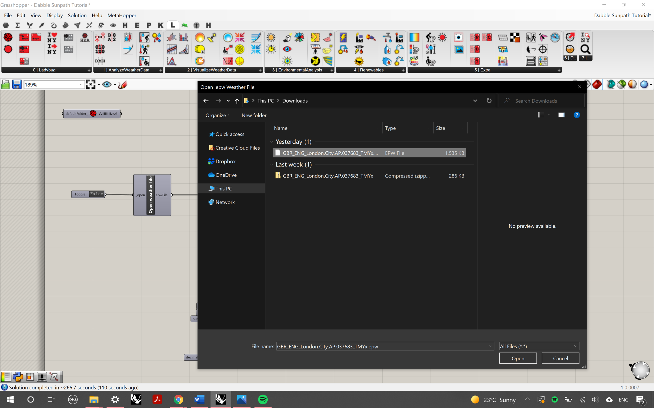
Once you’ve got all the sliders, zoom back out so you can see the toggle button. Double click on the black ‘false’ button on the component to turn it to true. This will trigger the command to open and import the EPW data from the file previously downloaded. Make sure you extract the correct file format (EPW) amongst the others in the ZIP Folder obtained from the EPW map site. Select this file and click open.


Minimise Grasshopper to see the sun path on your Rhino File. You can now place your proposal in the centre of the sun path and capture a view of it to show the sun’s position in relation to your project. For more aesthetic results, use the rendered option to get a more sleek look. You can do this by pressing space on the Rhino interface and typing in the ‘Rendered’ command to activate this view style.
Wind Rose
Step 1:
The first section of the wind rose script will be very similar to that of the sun path. Insert the following components and arrange as shown in the slide above:
Ladybug_Ladybug
Honeybee_Honeybee
Boolean Toggle
Open EPW File
Import EPW File
Connect the last three components in a line in the same order as they are listed.
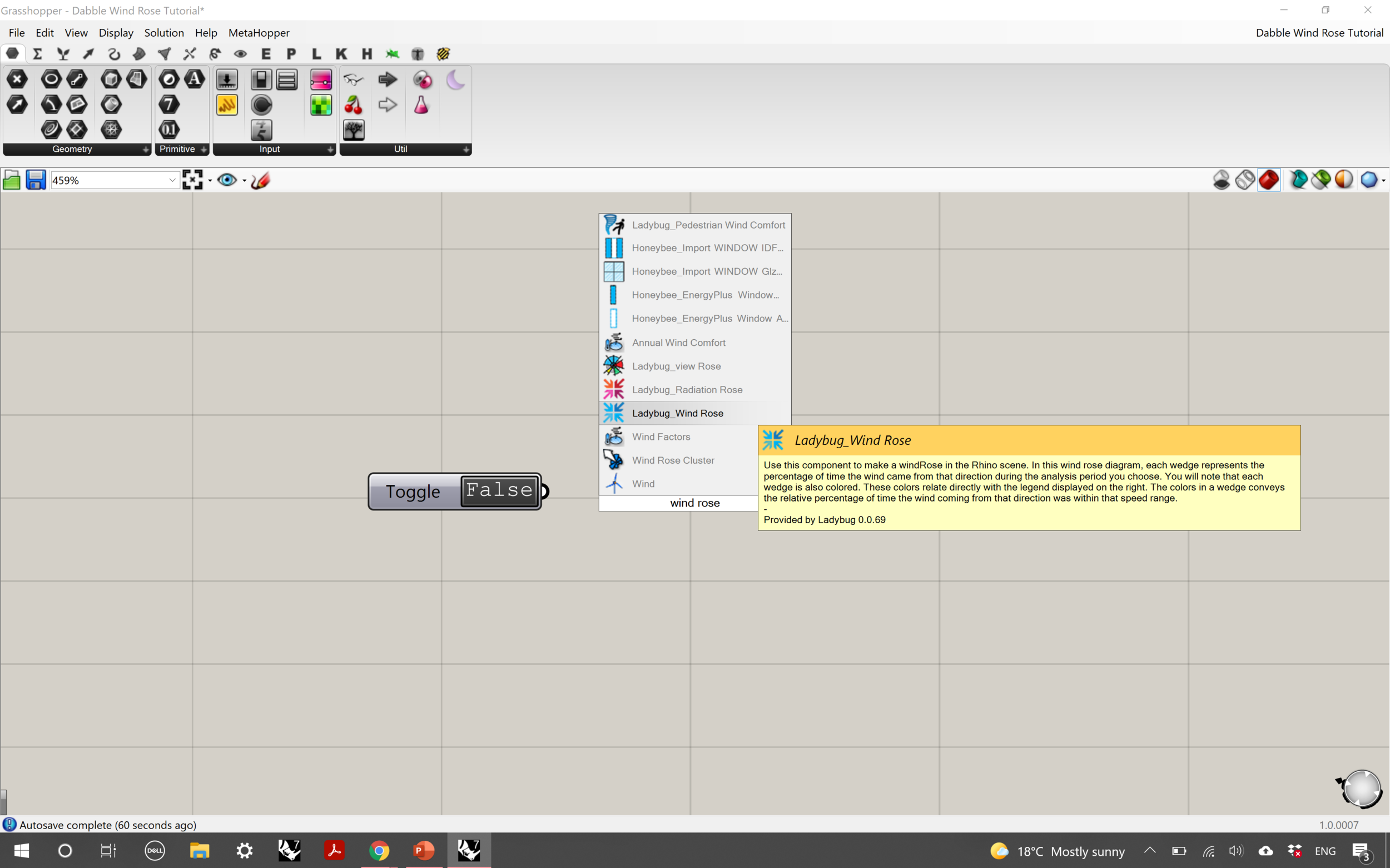

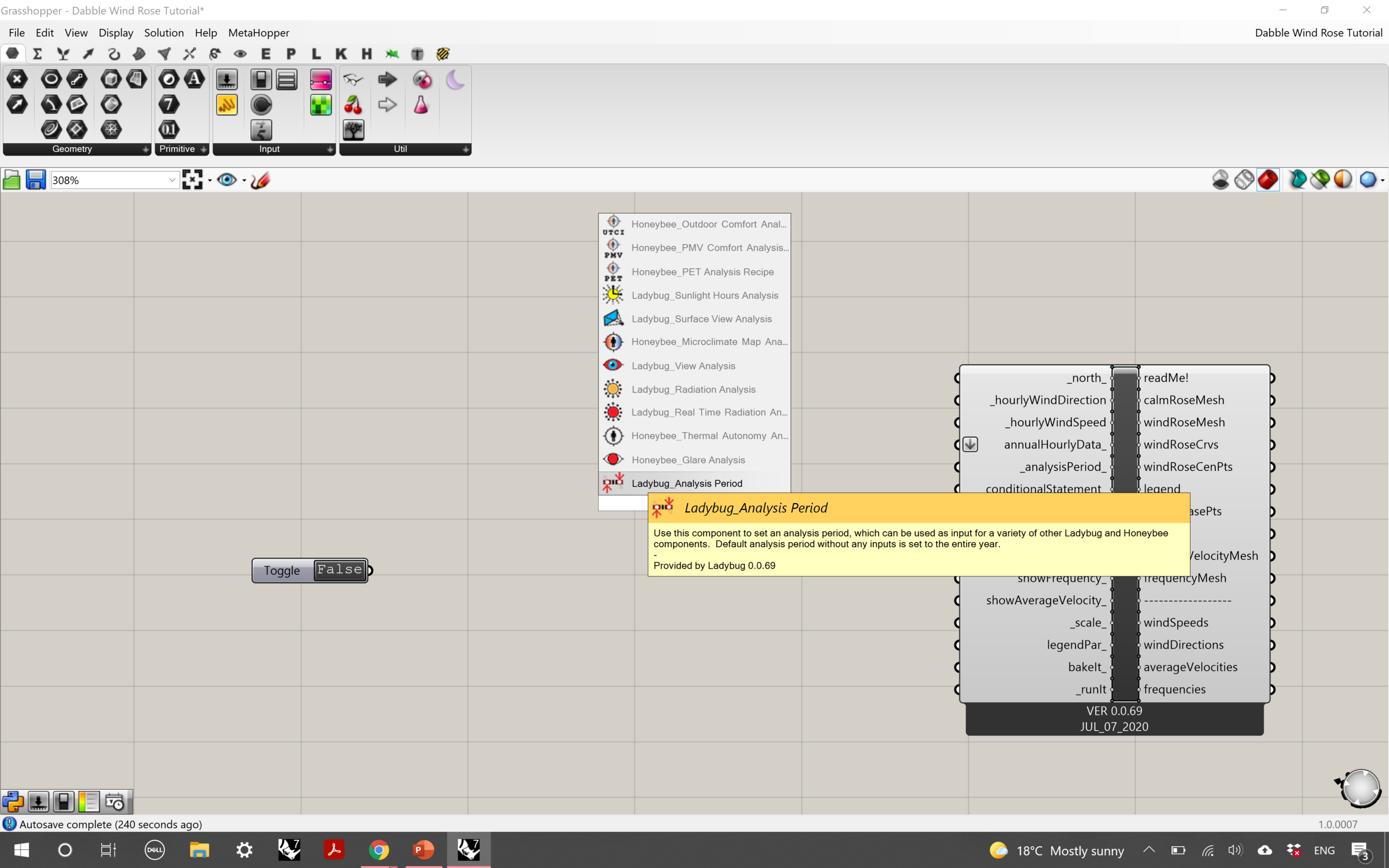

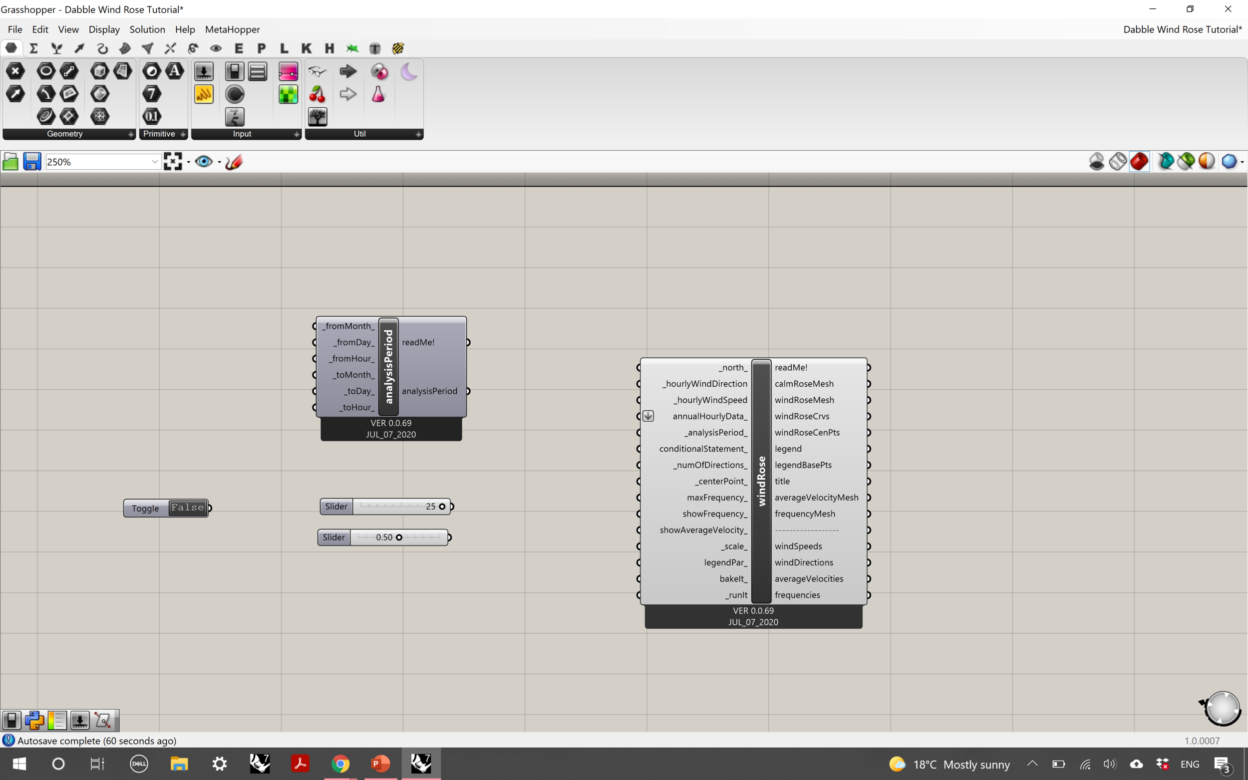


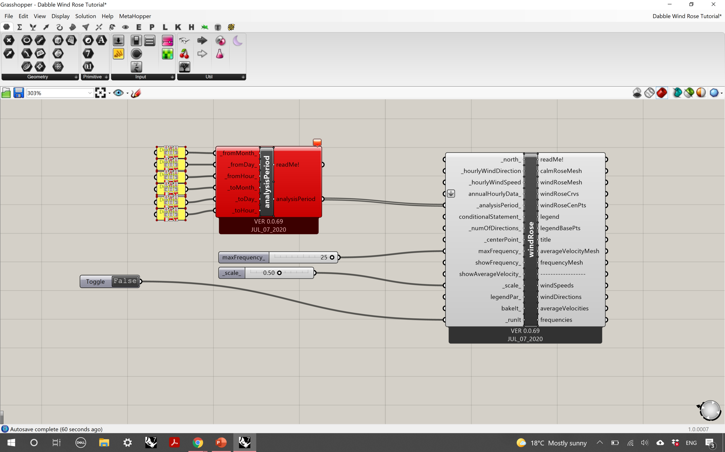

Step 2:
Move along your workspace to the right of the first few components of the script. Insert the ‘Boolean Toggle’, ‘Ladybug Windrose’ and ‘Ladybug Analysis Period’ components. You’ll also need two sliders, connecting to the maxFrequency and scale inputs of the wind rose component. These will have the following parameters:
Max frequency:
Decimal Points: 0
Min: 0
Max: 25
Scale:
Decimal Points: 2
Min: 0
Max: 1
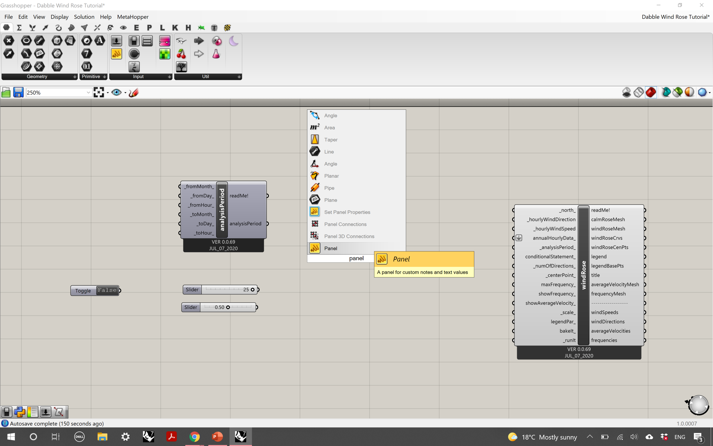
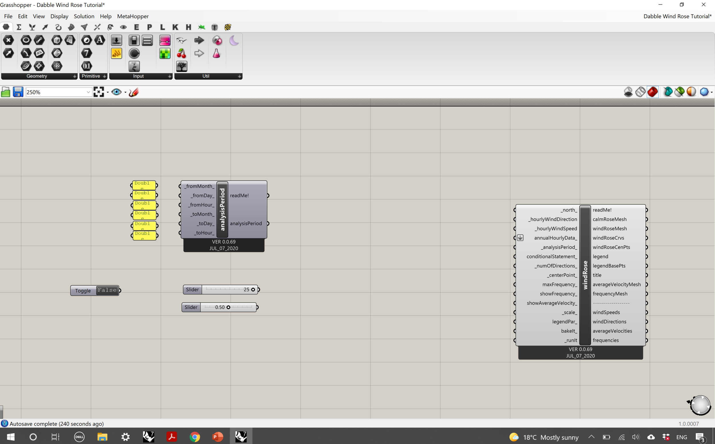
Insert 6 ‘Panel’ components and place them so they correspond to the 6 inputs of the analysis period component. This is where you’ll be inputting the time frame which your wind rose represents.
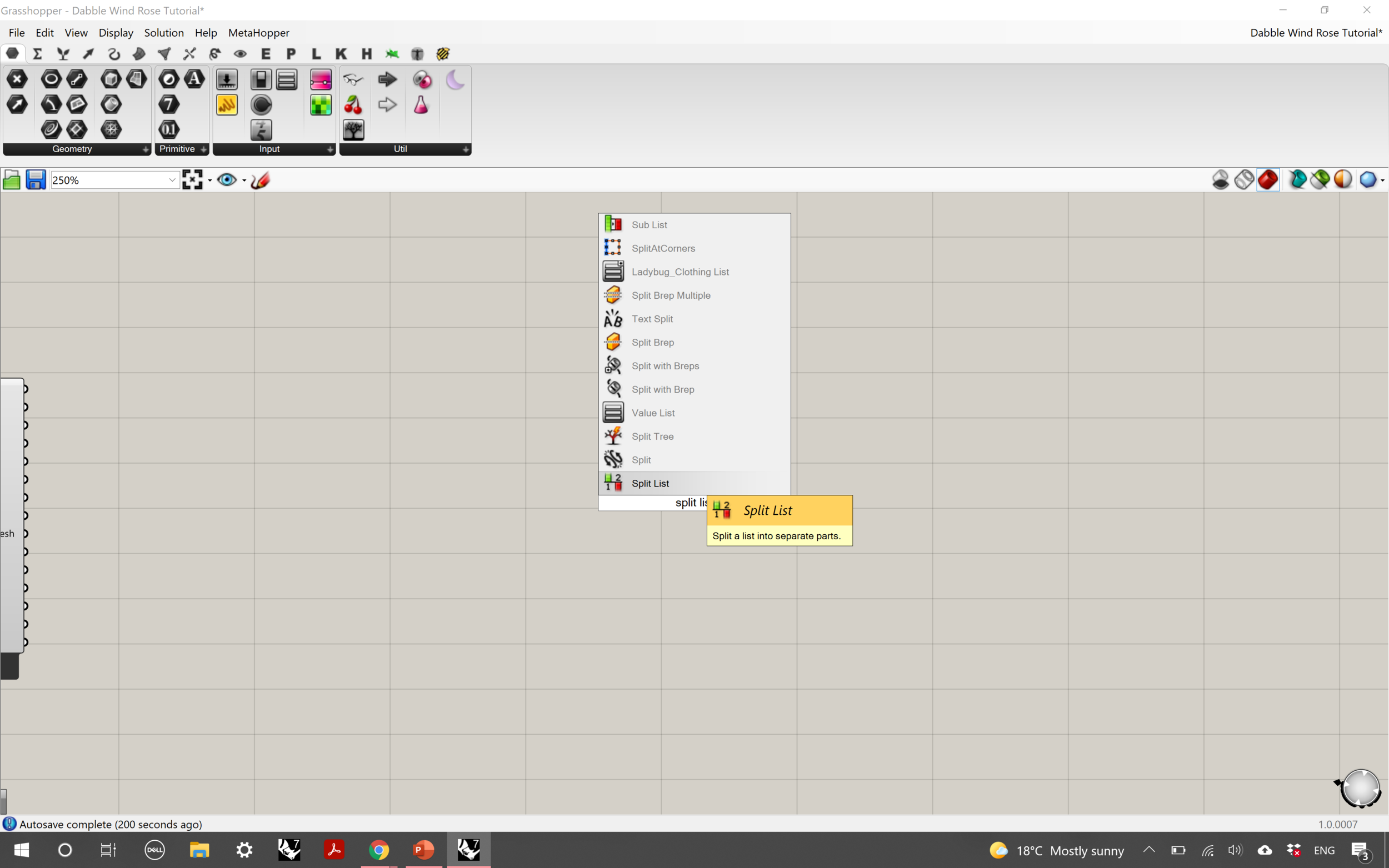


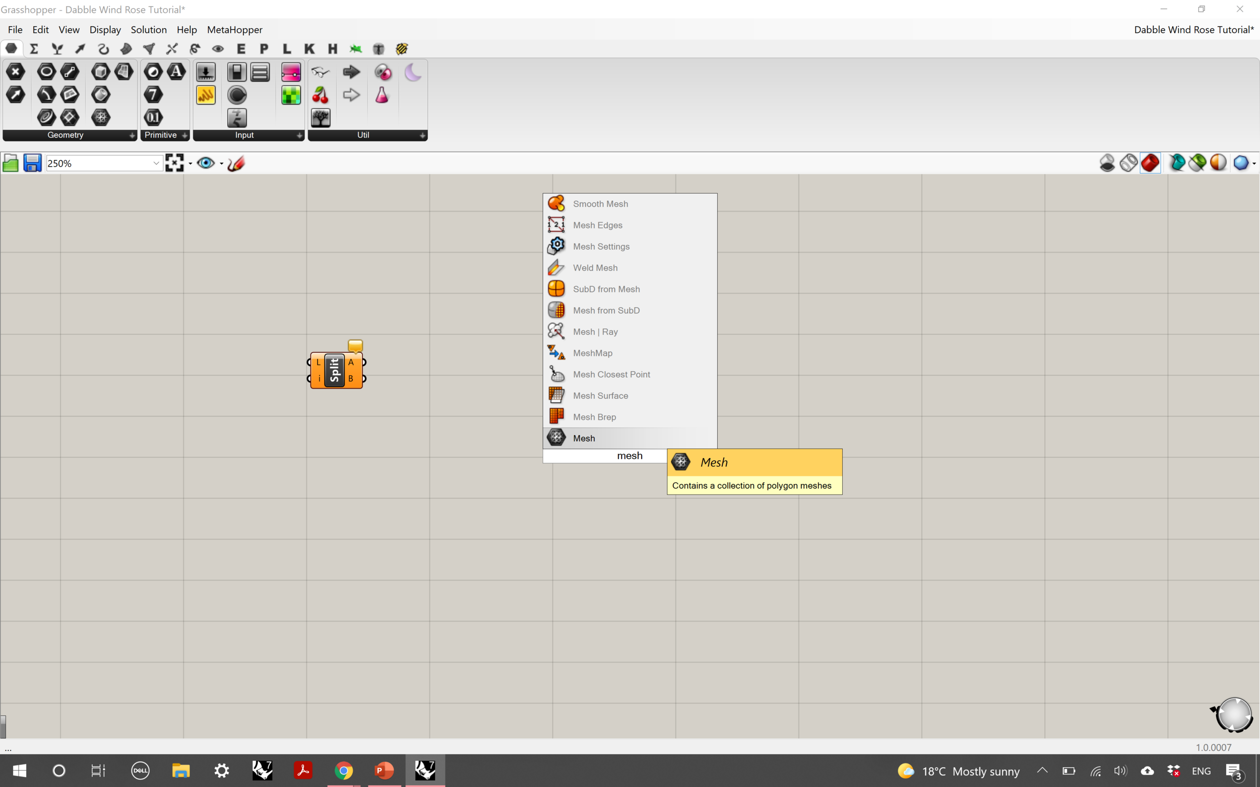

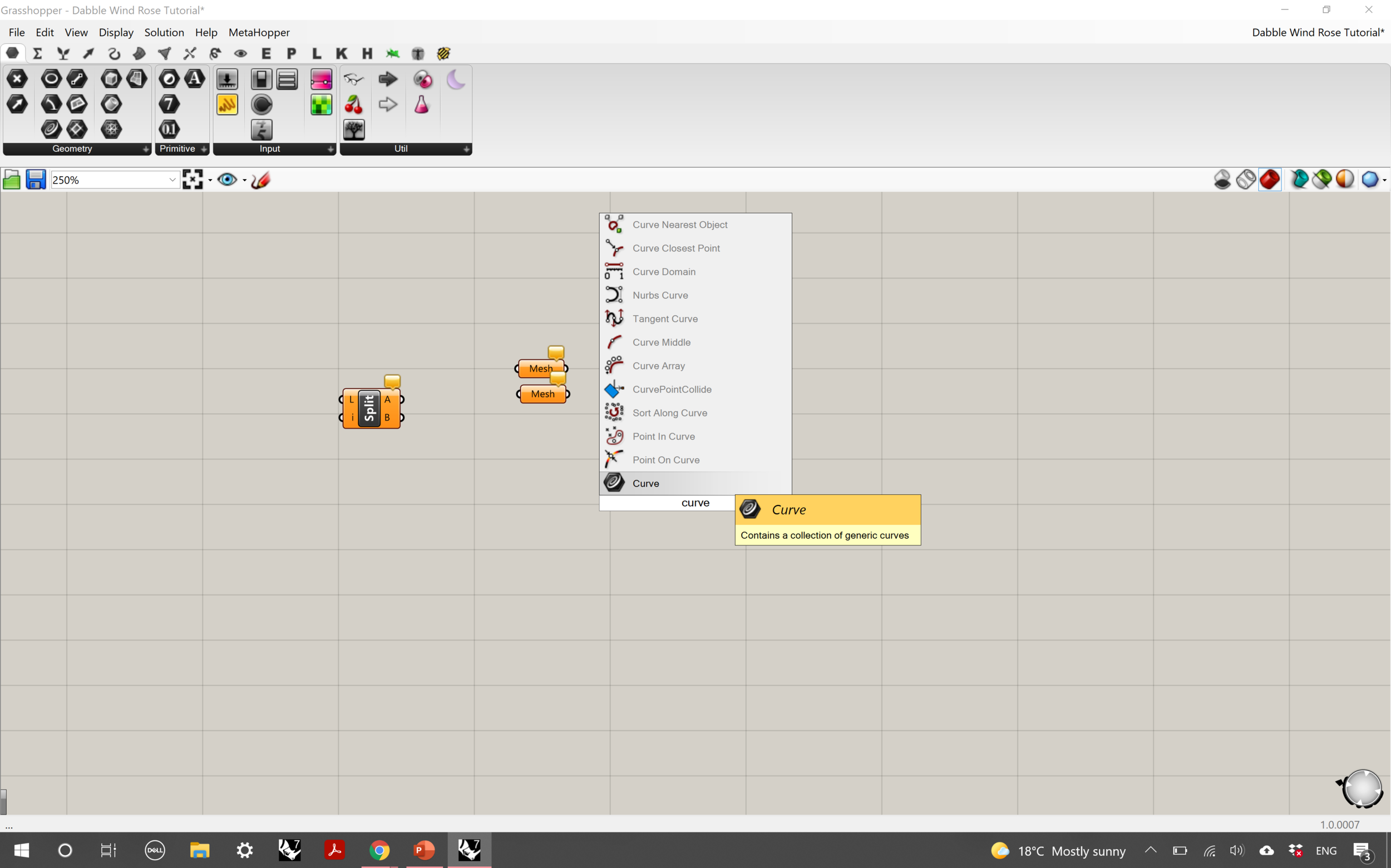

Step 3:
Once again, move along to the right of the components you worked on. Insert these components onto the workspace:
Split List
2 Mesh components
1 curve component


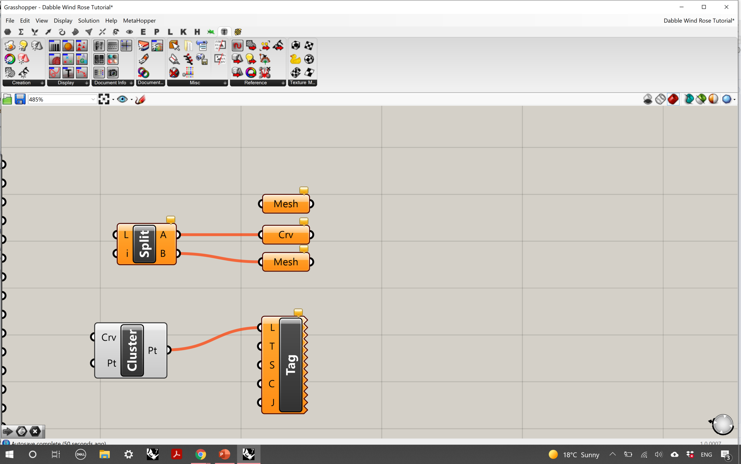

Next, we’re going to be combining certain components to make a cluster.
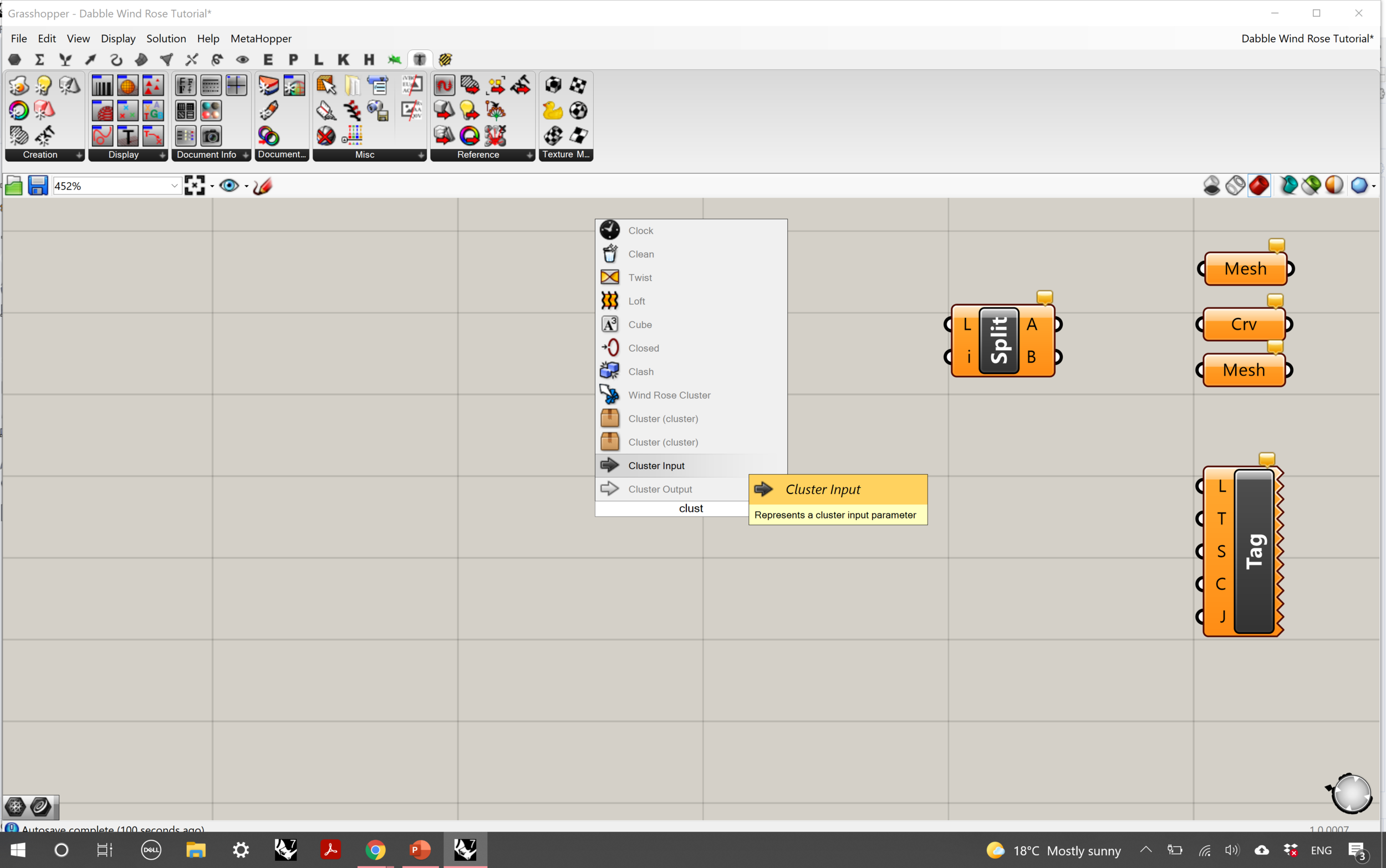
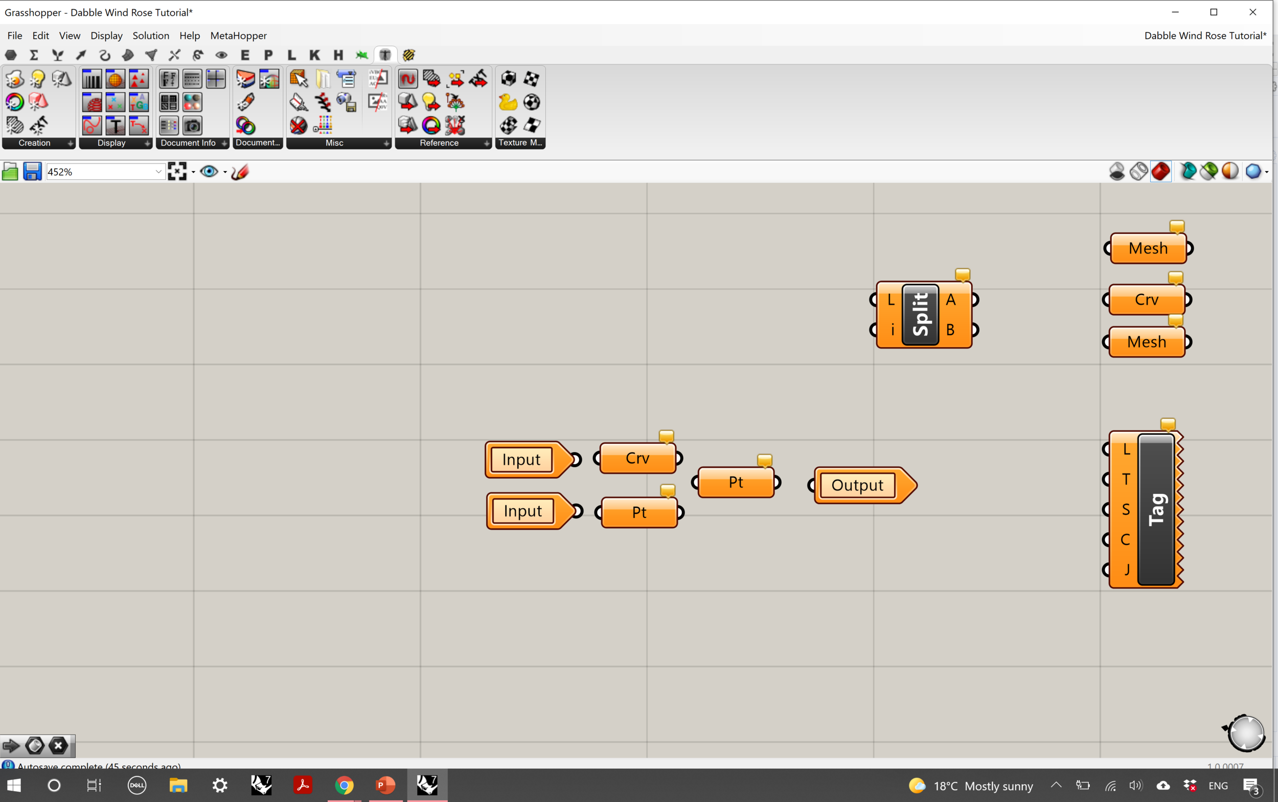
Insert two ‘Cluster Inputs’ and place one above the other in a line. Place a ‘Curve’ component next to the top ‘Cluster Input’, and a ‘Point component’ next to the bottom cluster input.
Place a second ‘Point’ to the right of these components, and a ‘Cluster Output’ component next to this.
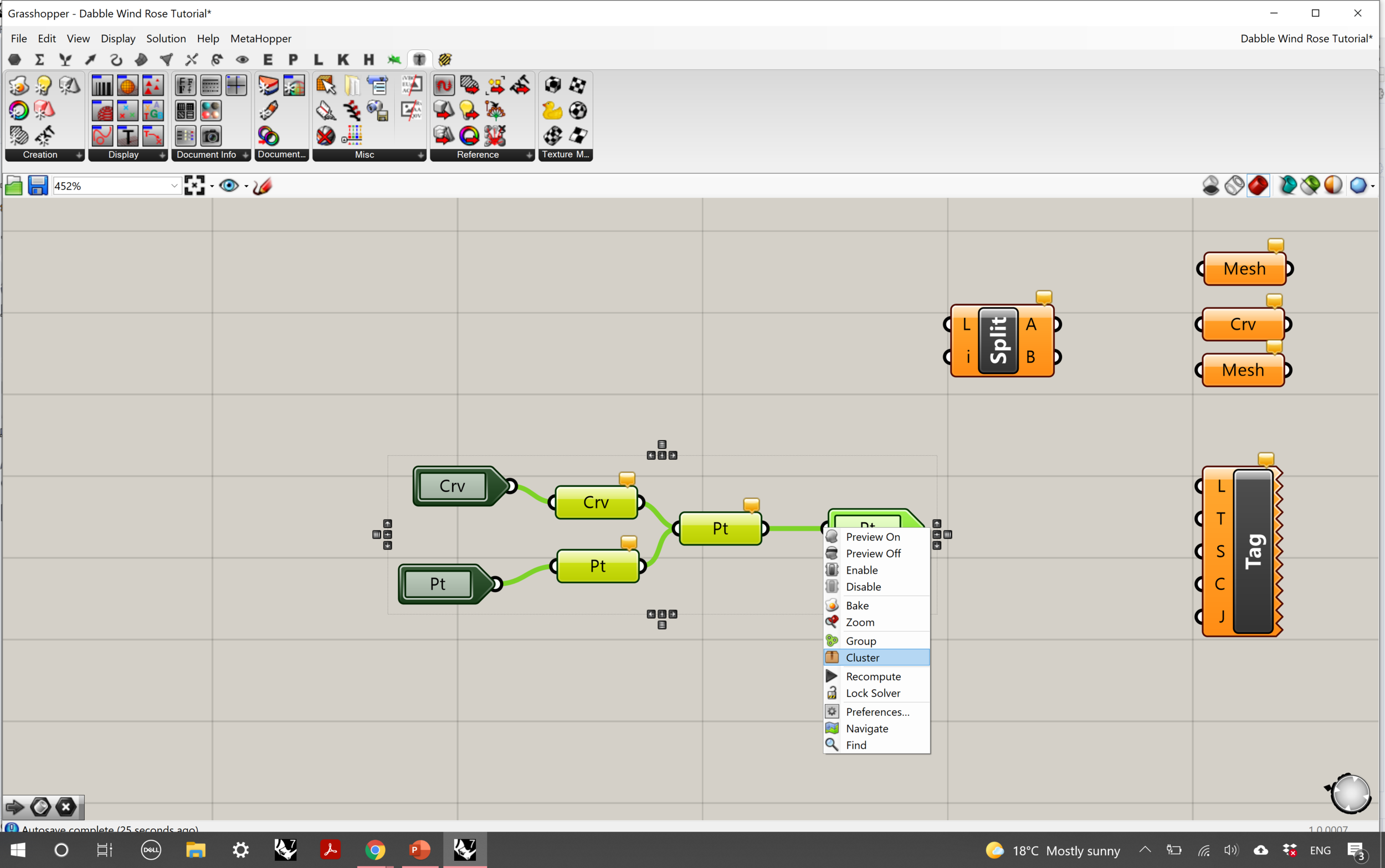
Select these components, right-click on one of the white semi-circles on the side of a component, and click ‘Cluster’. You should now have one single component that combines the ones you just inserted and connected in your workspace.
Step 4:
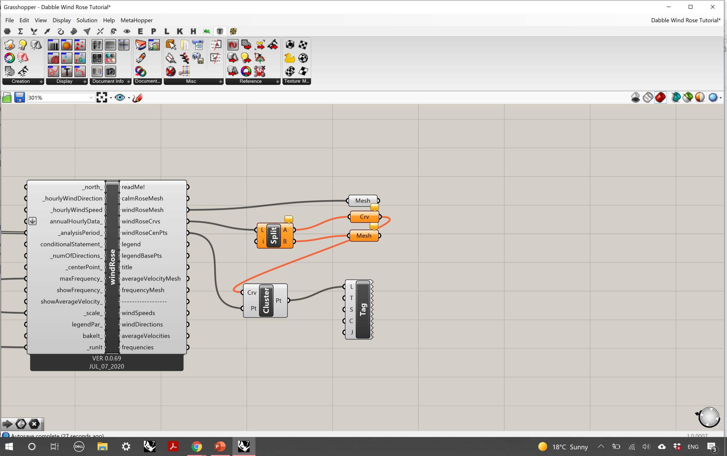
The following steps requires connecting the different parts of the script together.
Connect the following together:
windRoseMesh (windRose) -> Mesh
windRoseCrvs (windRose) -> Split L input
windRoseCentPts (windRose) -> Cluster Pt input
Split A output -> Curve
Split B output -> Mesh
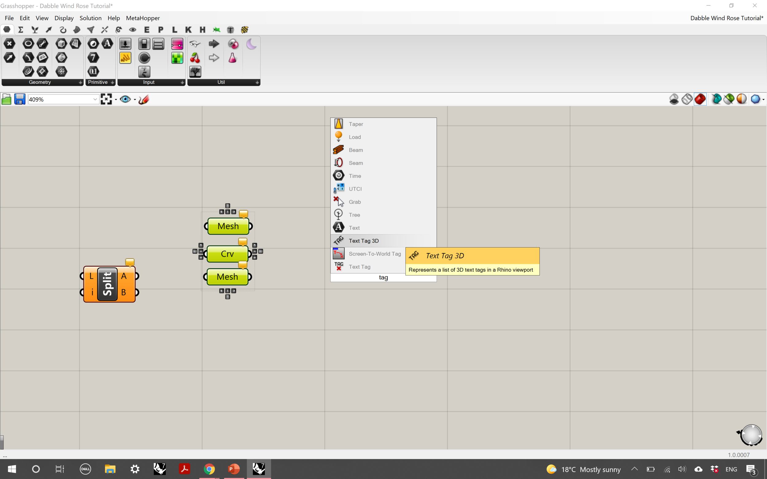
Cluster Pt output -> Tag L input
Cluster Crv input -> Crv output
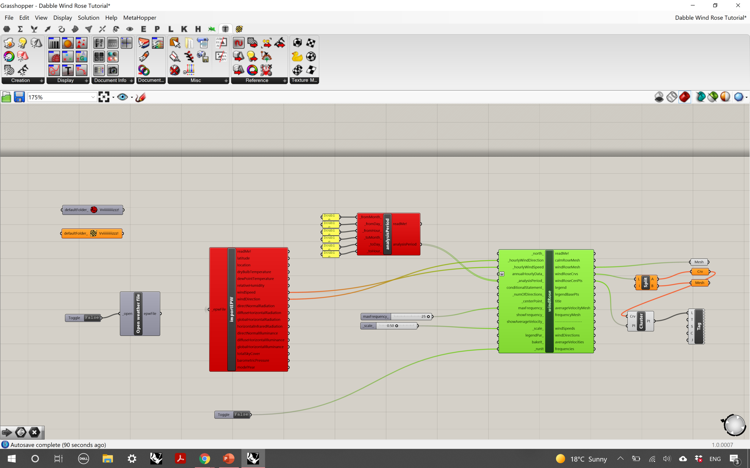
Step 5:
Next, make these following connections:
AnalysisPeriod (analysisPeriod) -> analysisPeriod (windRose)
windSpeed (importEPW) -> hourlyWindSpeed (windRose)
windDirection (importEPW) -> hourlyWindDirection (windRose)
Slider 1 -> maxFrequency (windRose)
Slider 2 -> scale (windRose)
Boolean Toggle - runIt (windRose)
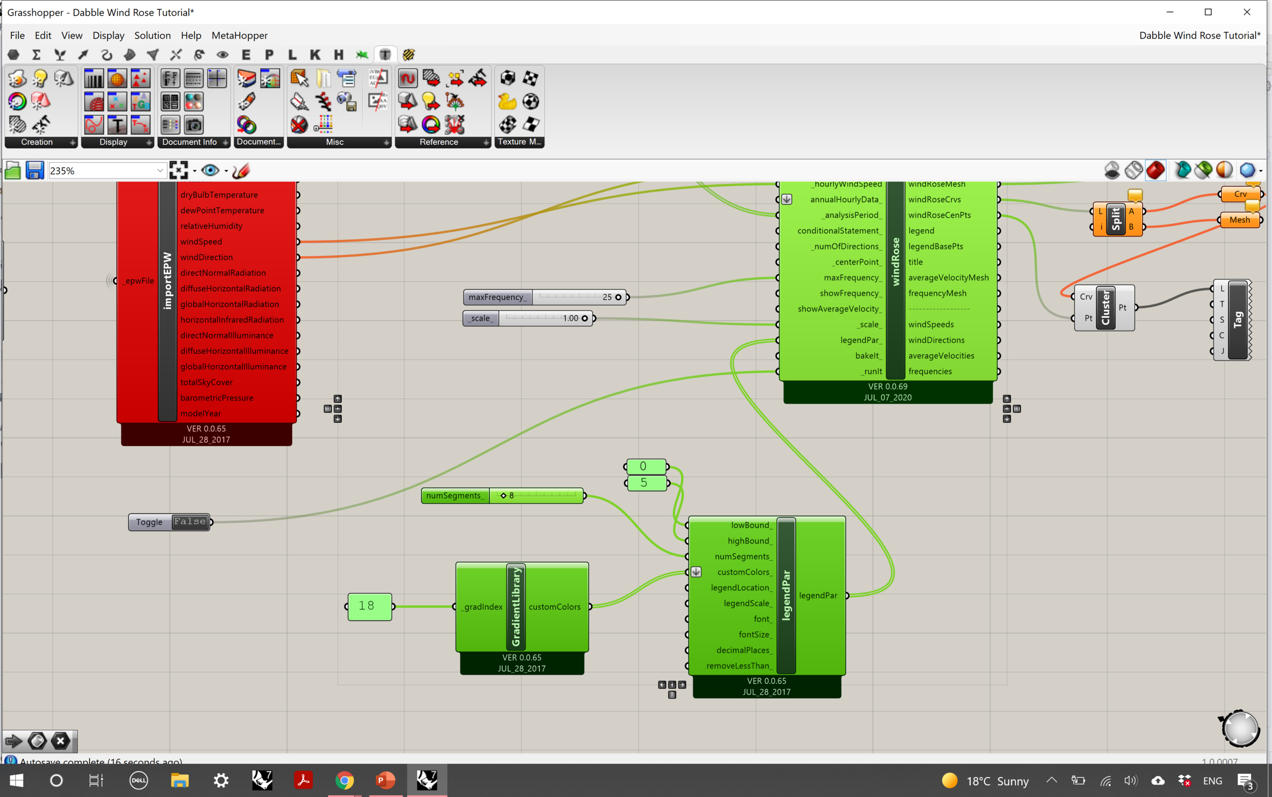
Step 6:
To create the legend for the wind rose, you’ll need to recreate this section of the script highlighted in green. Connect these components in the following order:
Panel -> GradientLibrary -> customColours input of LegendPar Component -> legendPar input of windRose component.
Slider -> numSegments input of LegendPar component
Panel -> lowBound (legendPar)
Panel -> highBound (legendPar)
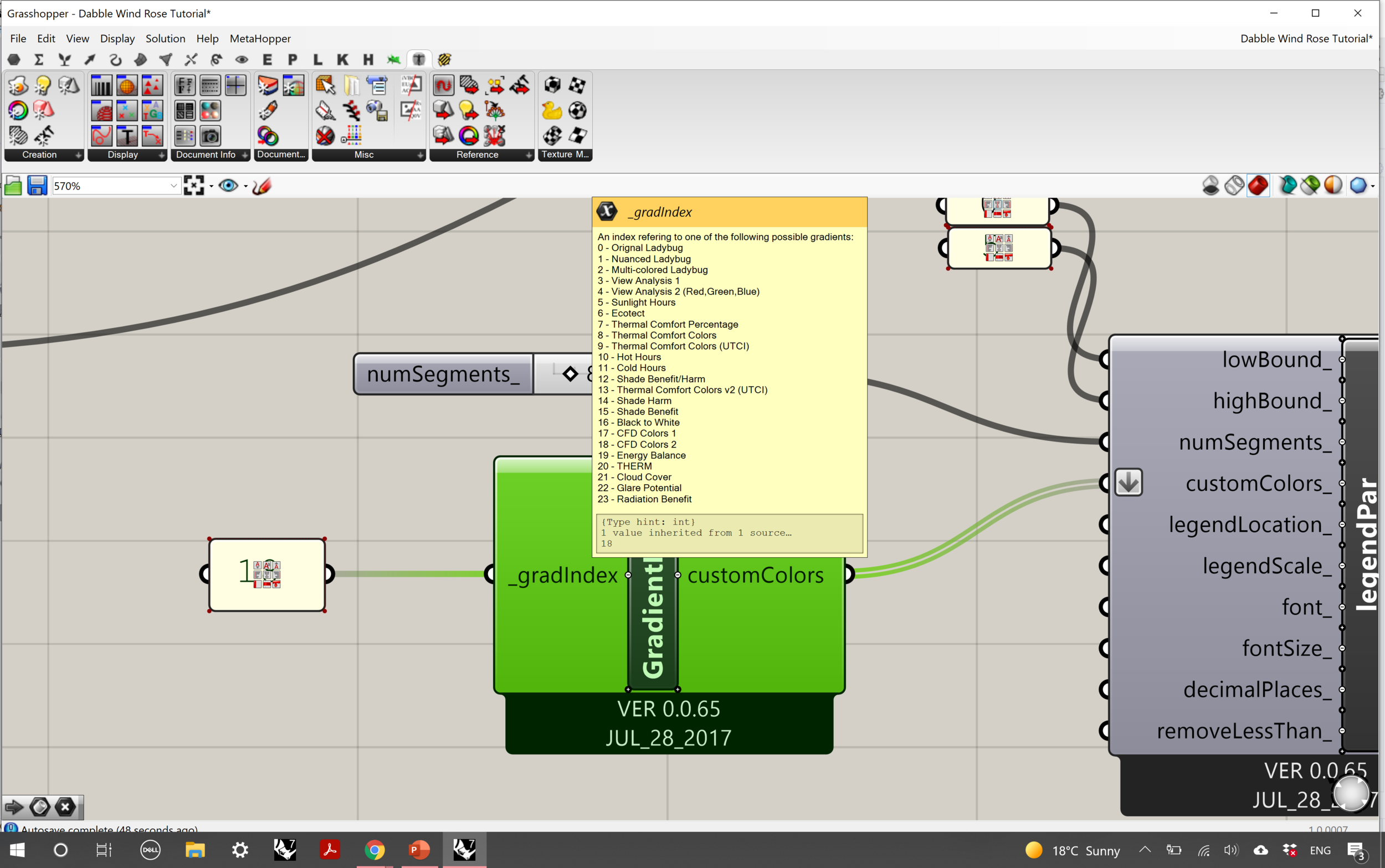
For the Gradient index panel input, hover over the ‘_gradIndex’ area of the panel to see the corresponding colour options. Some of these refer to environmental design guide conventions and standards, so bear this in mind when choosing the colour scheme of your wind rose.
Step 7:
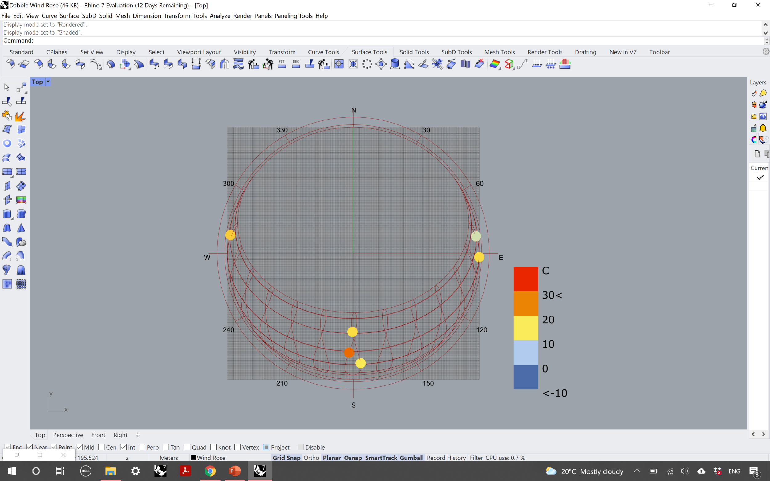
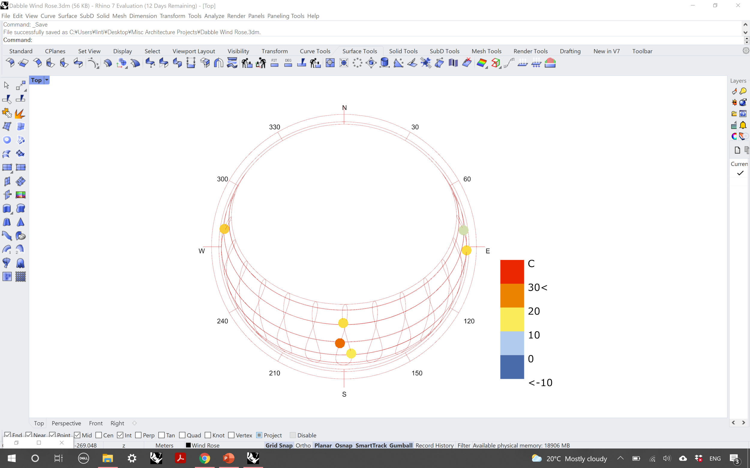
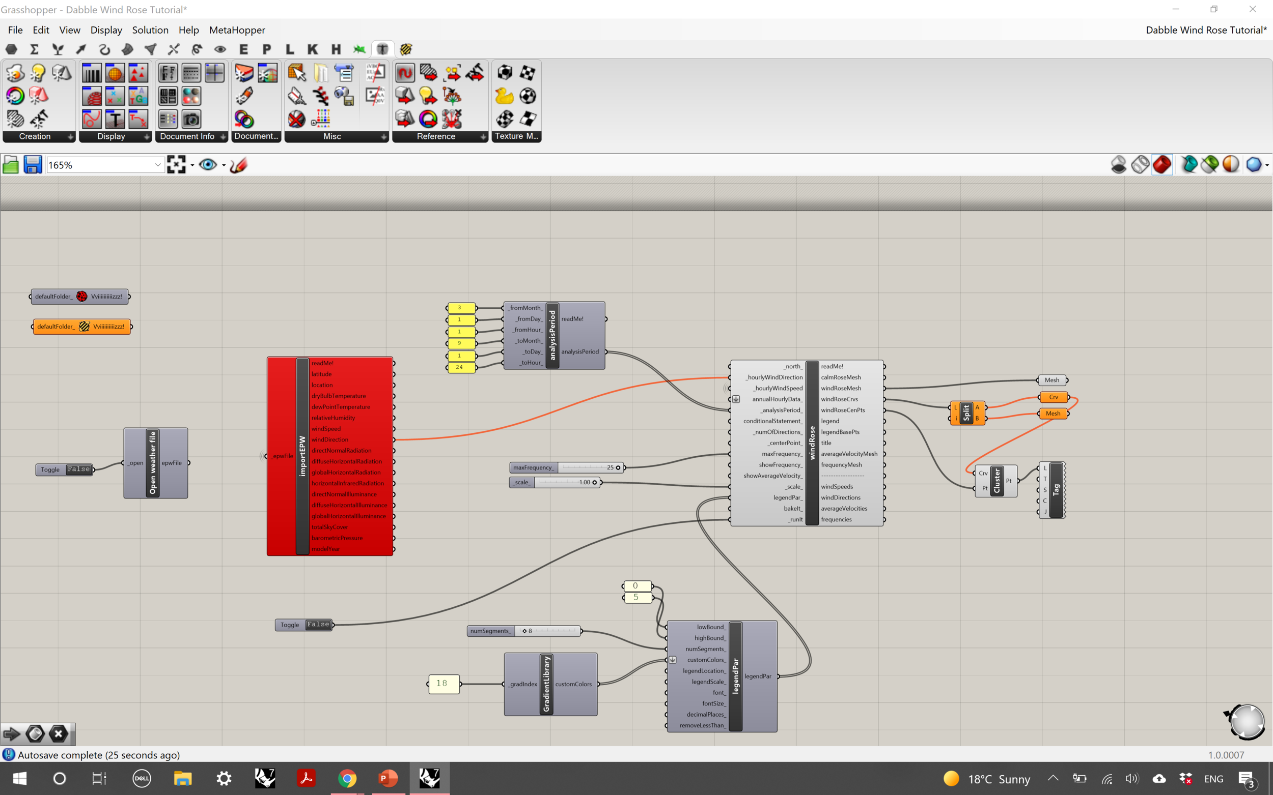
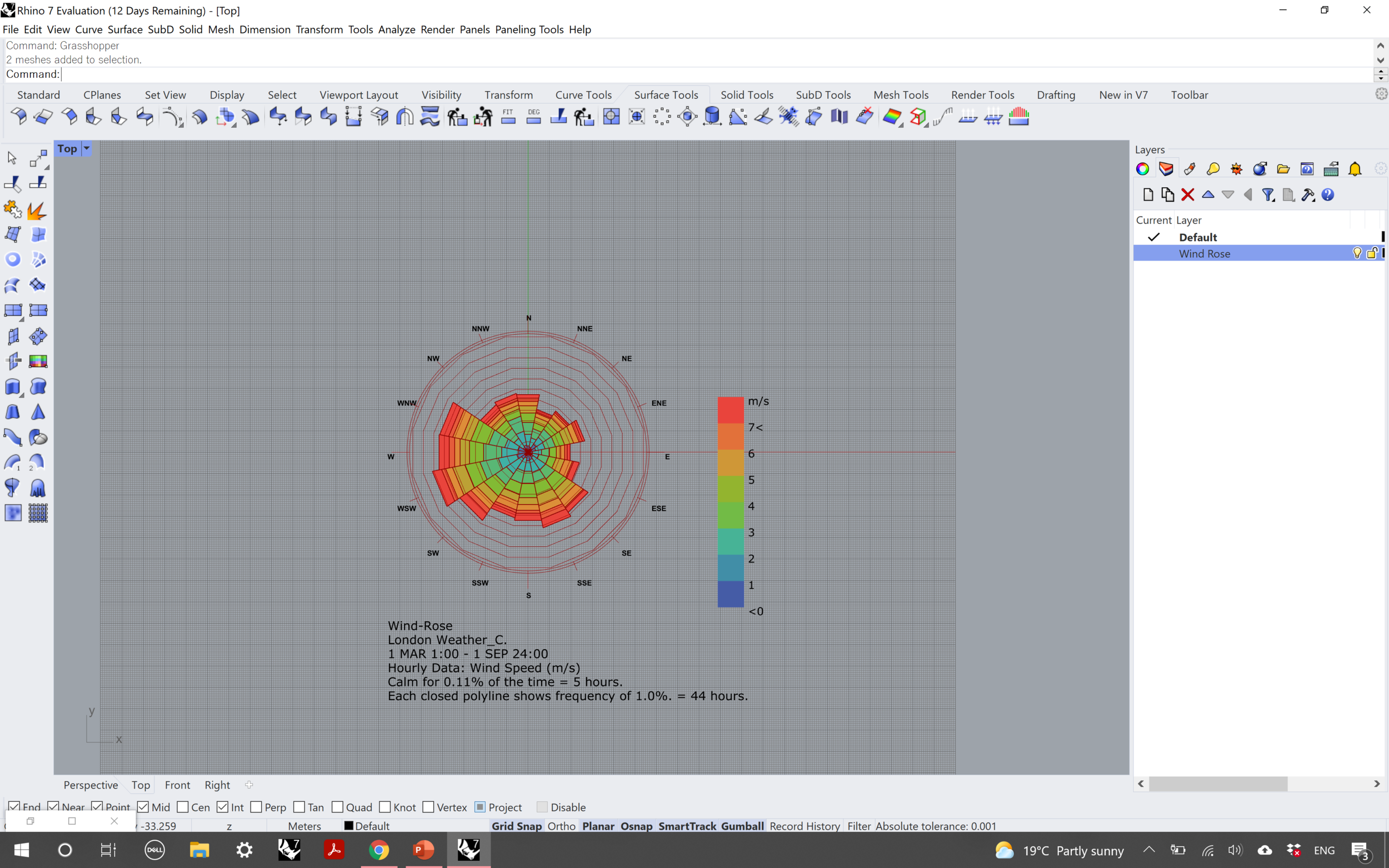
This is what your completed script should look like. Toggle both boolean toggles to true, select the EPW file when prompted as you did for the sun path, and minimise Grasshopper to see the result on Rhino.
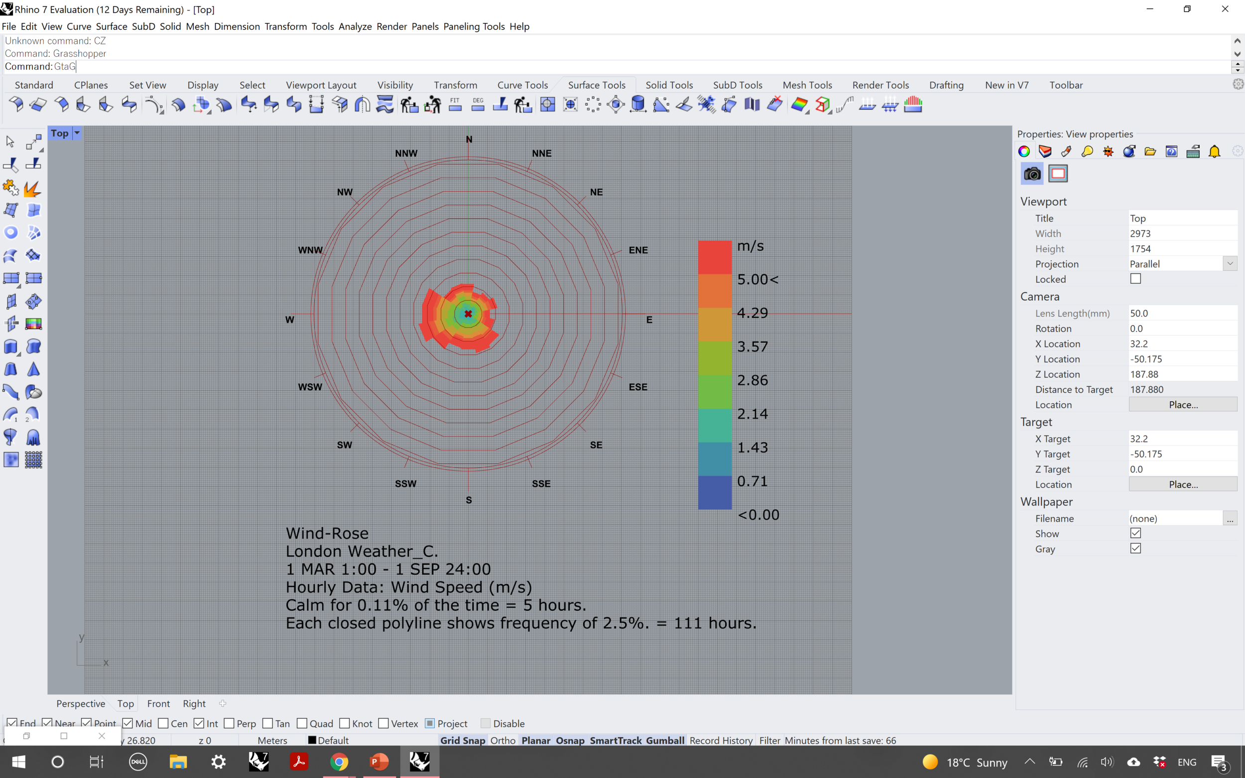


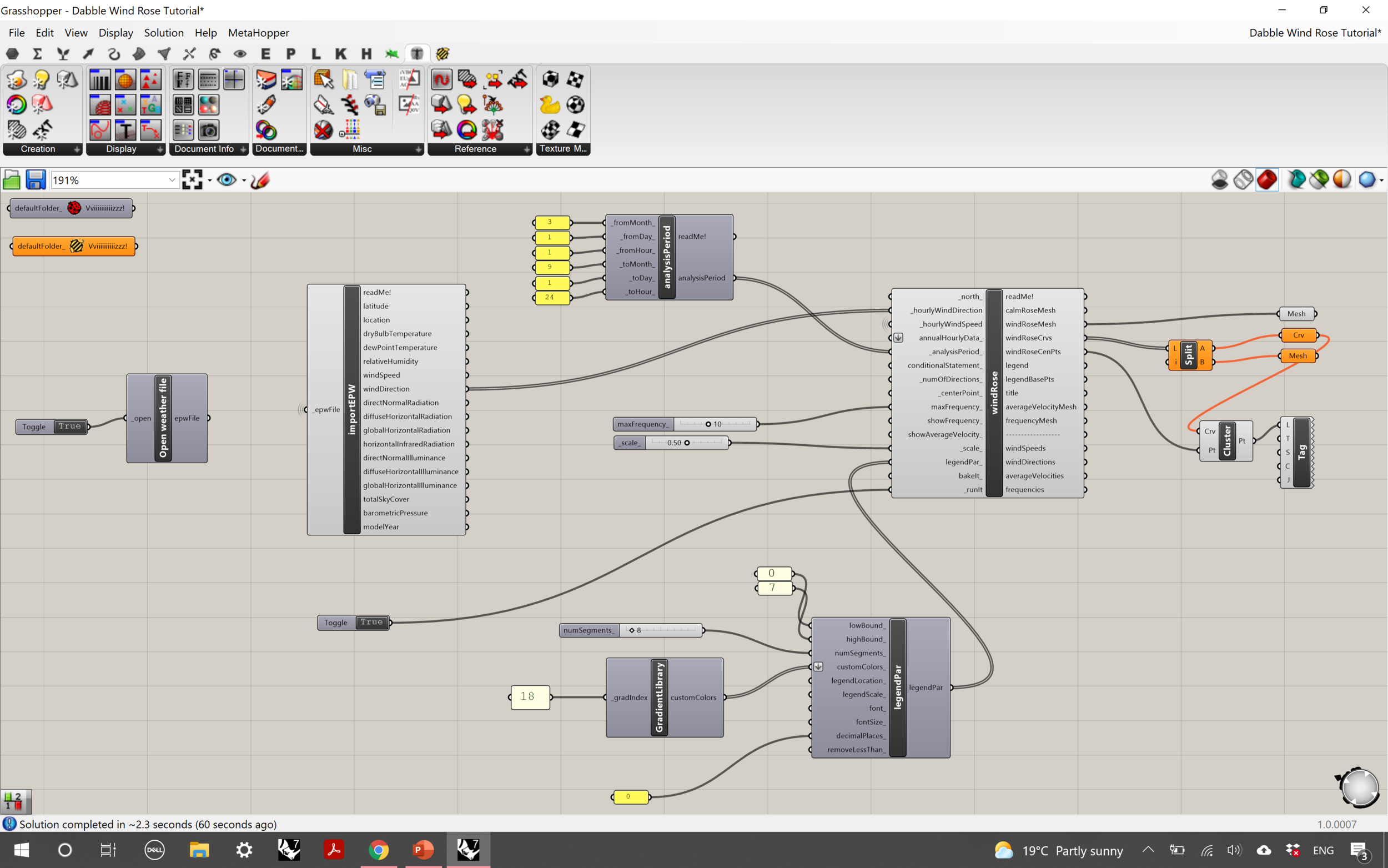
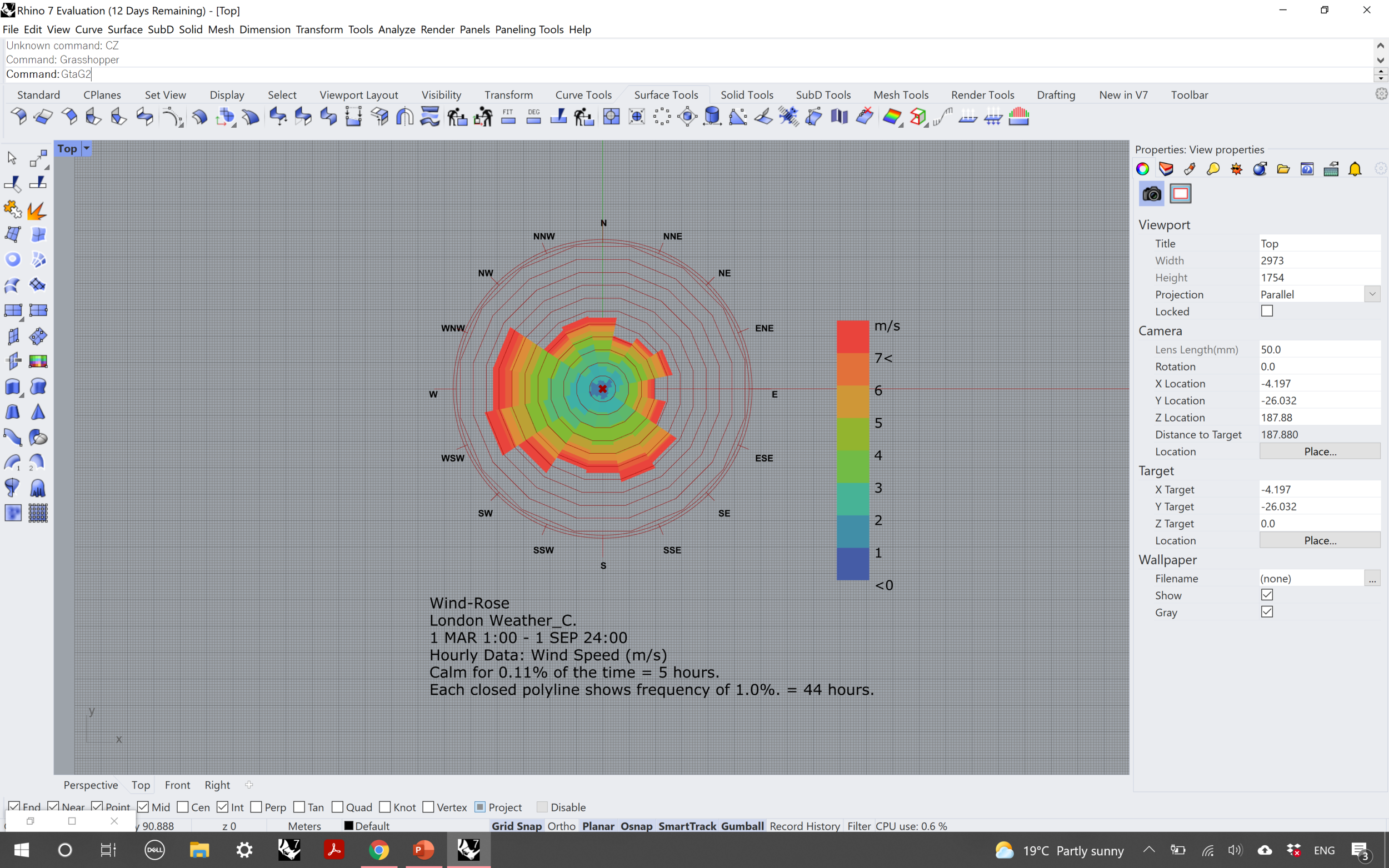

As you can see, initially some of the values needed to be tweaked to refine the wind rose. I added an extra panel to connect to the ‘decimalplaces’ input of the ‘legendPar’ component and set it to zero so that the key doesn’t have decimal places, and subsequently amended the segment number of the legend. I also brought down the ‘maxFrequency’ value so the wind rose itself was mapped out at an appropriate scale in comparison to the chart.


Step 8:
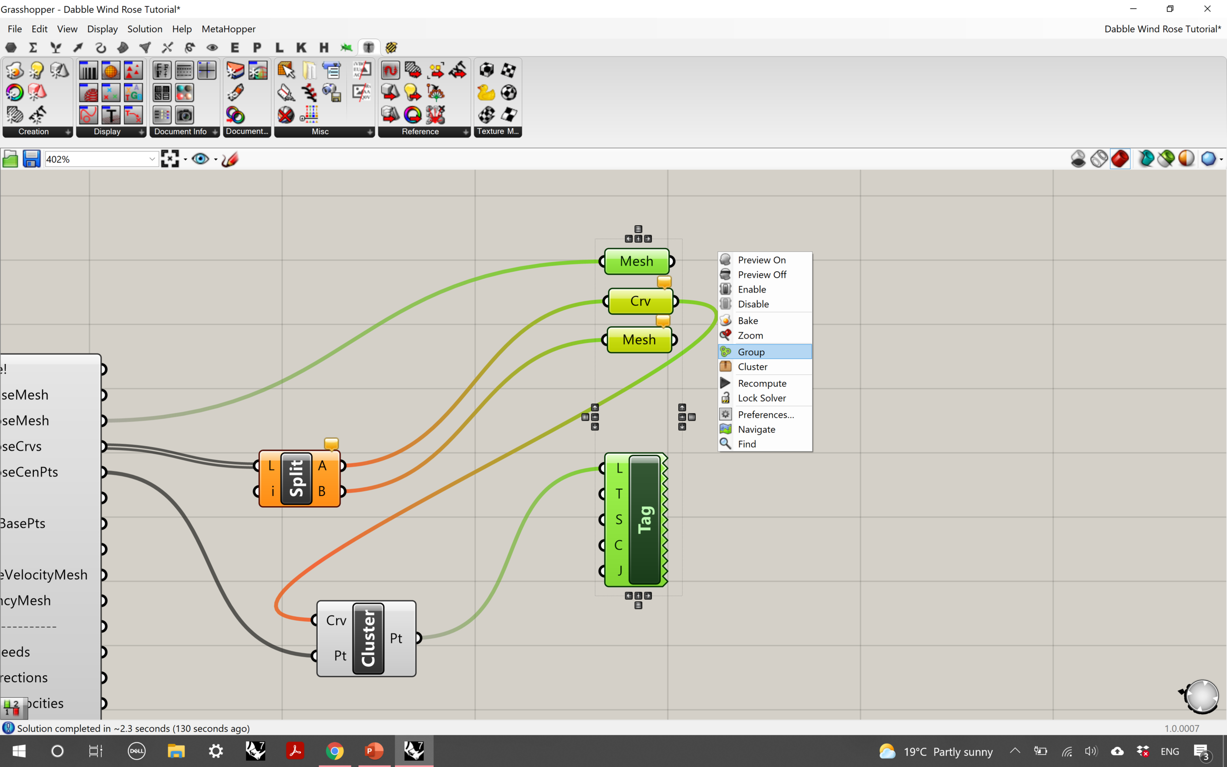
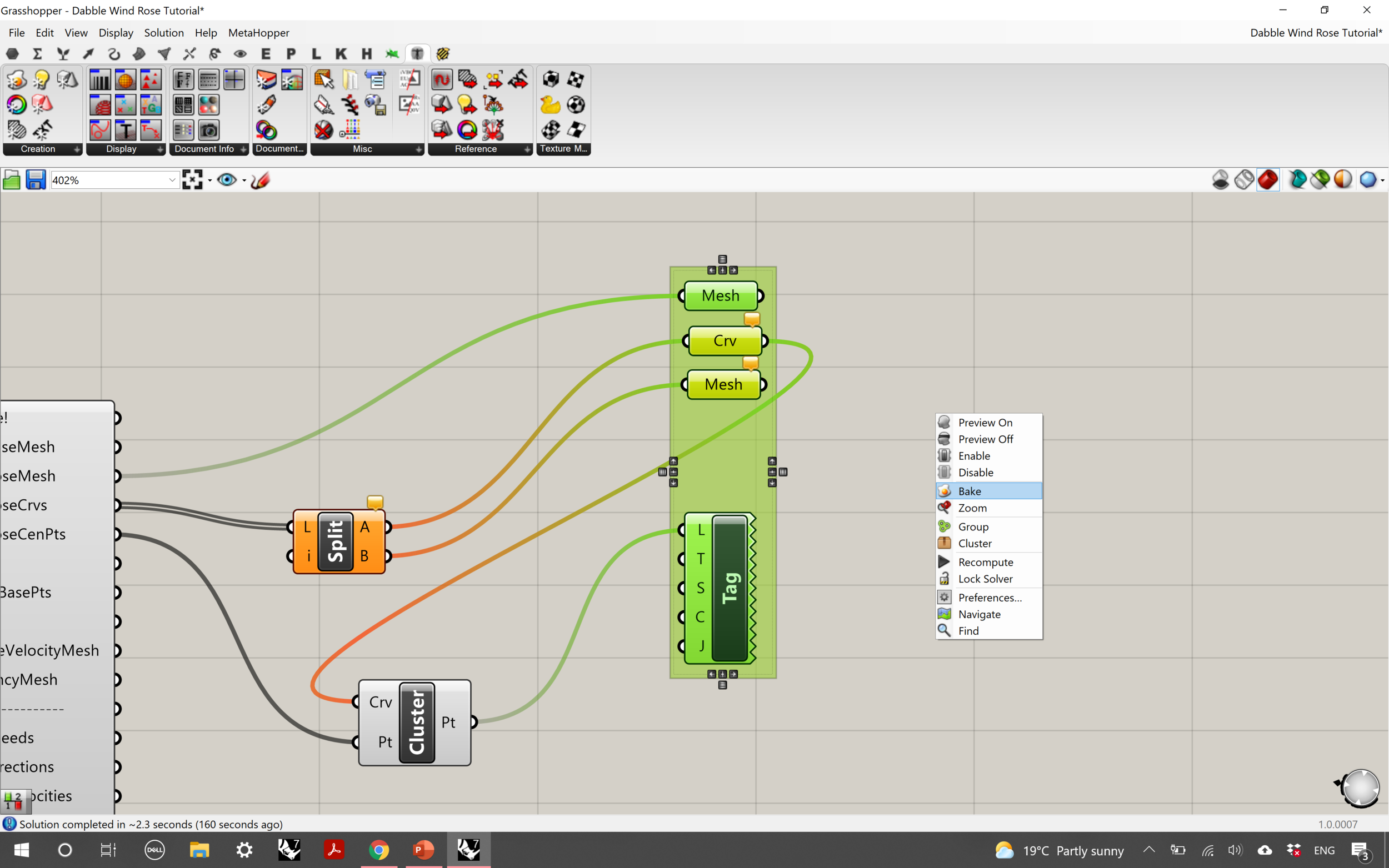
Next, we’re going to group and bake part of the script to turn the wind rose into a useable geometry on your Rhino file.
Select the ‘Mesh’, ‘Curve’ and ‘Tag’ components at the end of the script, right click on the workspace and select group. Then, select the newly made group, right click on the workspace again and choose ‘Bake’.
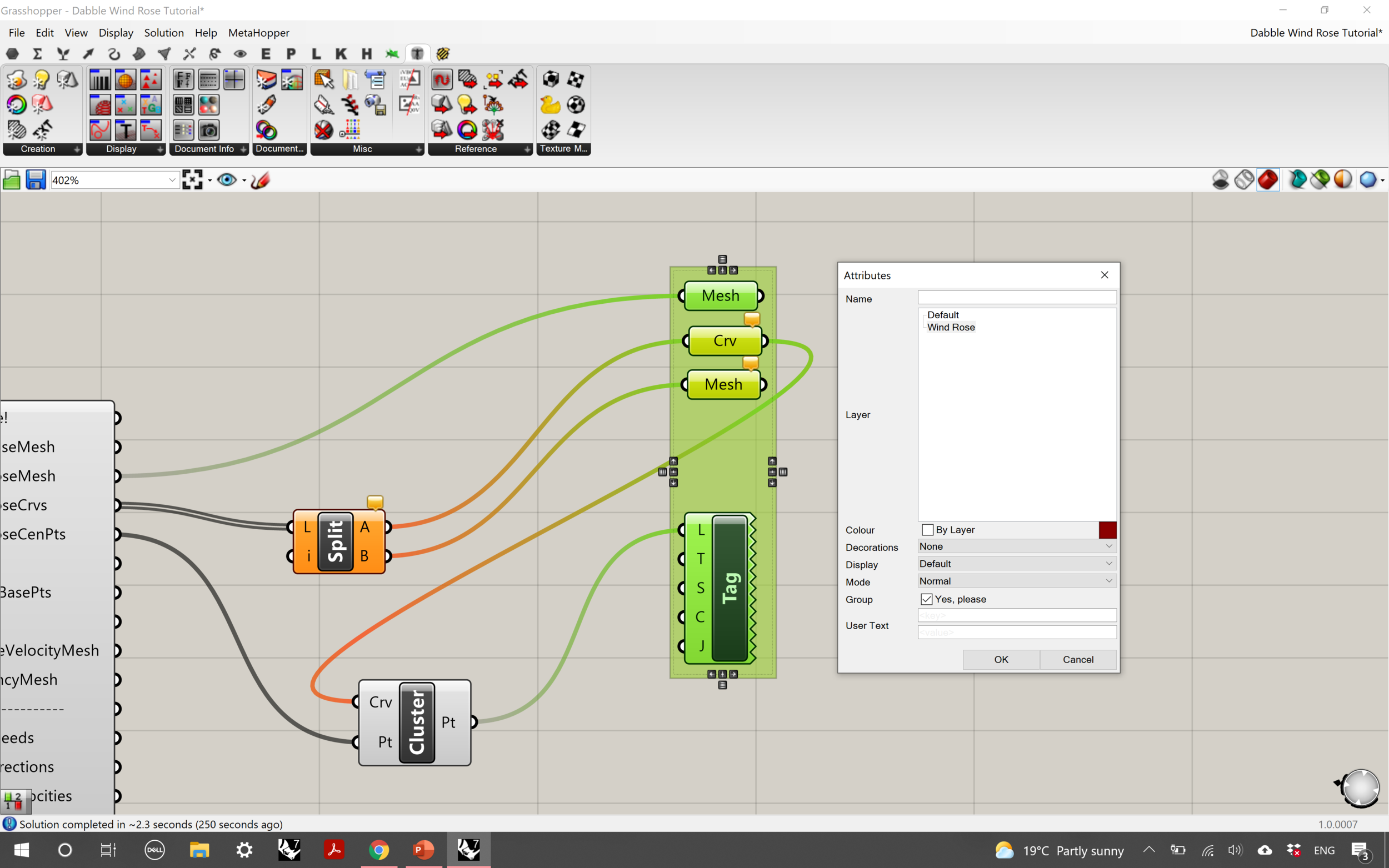
In the pop-up window, select a separate layer for the wind rose components (I previously made a separate one beforehand) on your Rhino file, untick the ‘Colour: By Layer’ box, tick the ‘Group: Yes, please’ box and click ‘OK’.
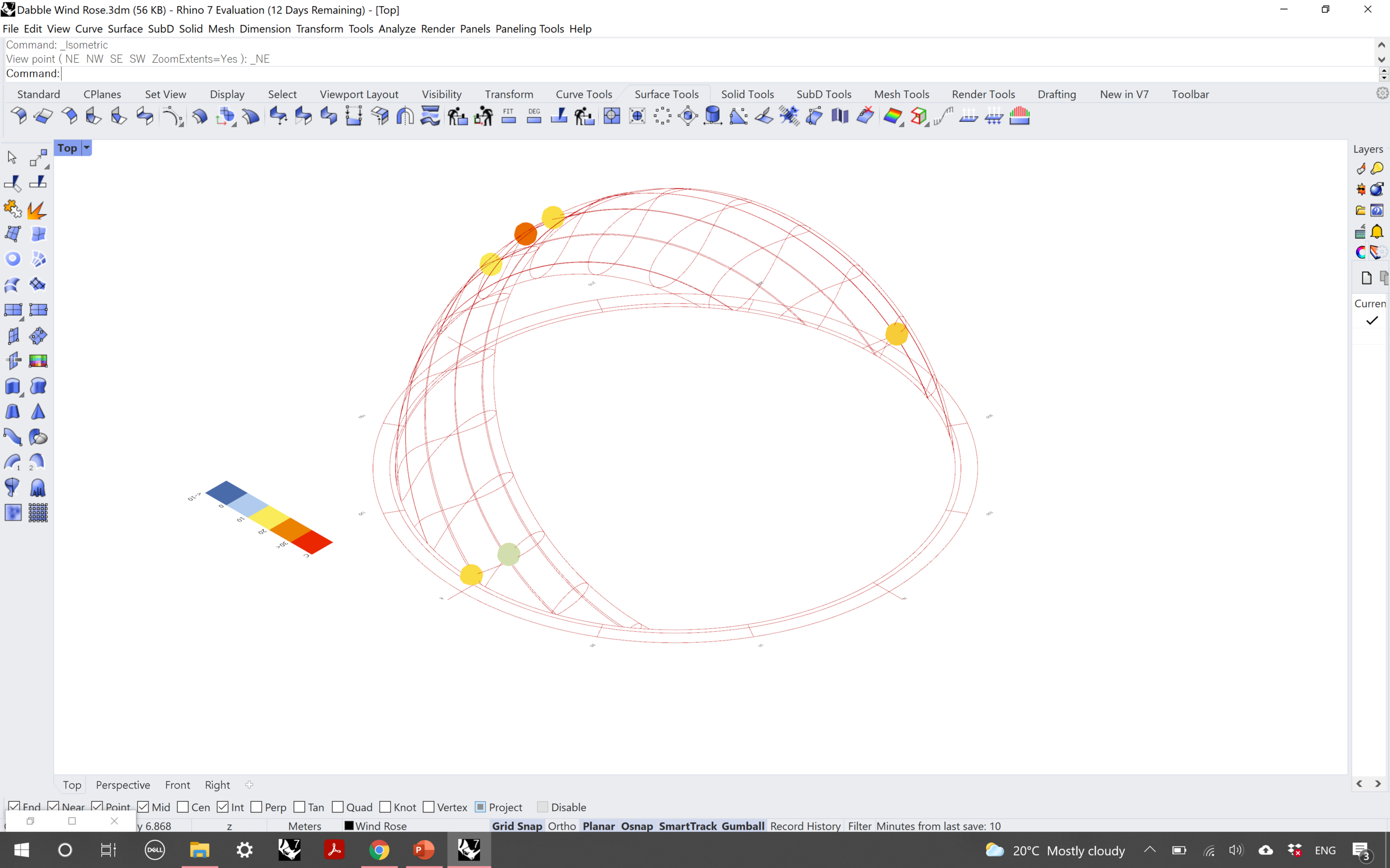
Return to your Rhino file. You should see that the wind rose itself can be moved around, which makes it easy for you to apply it to your site analysis representations.
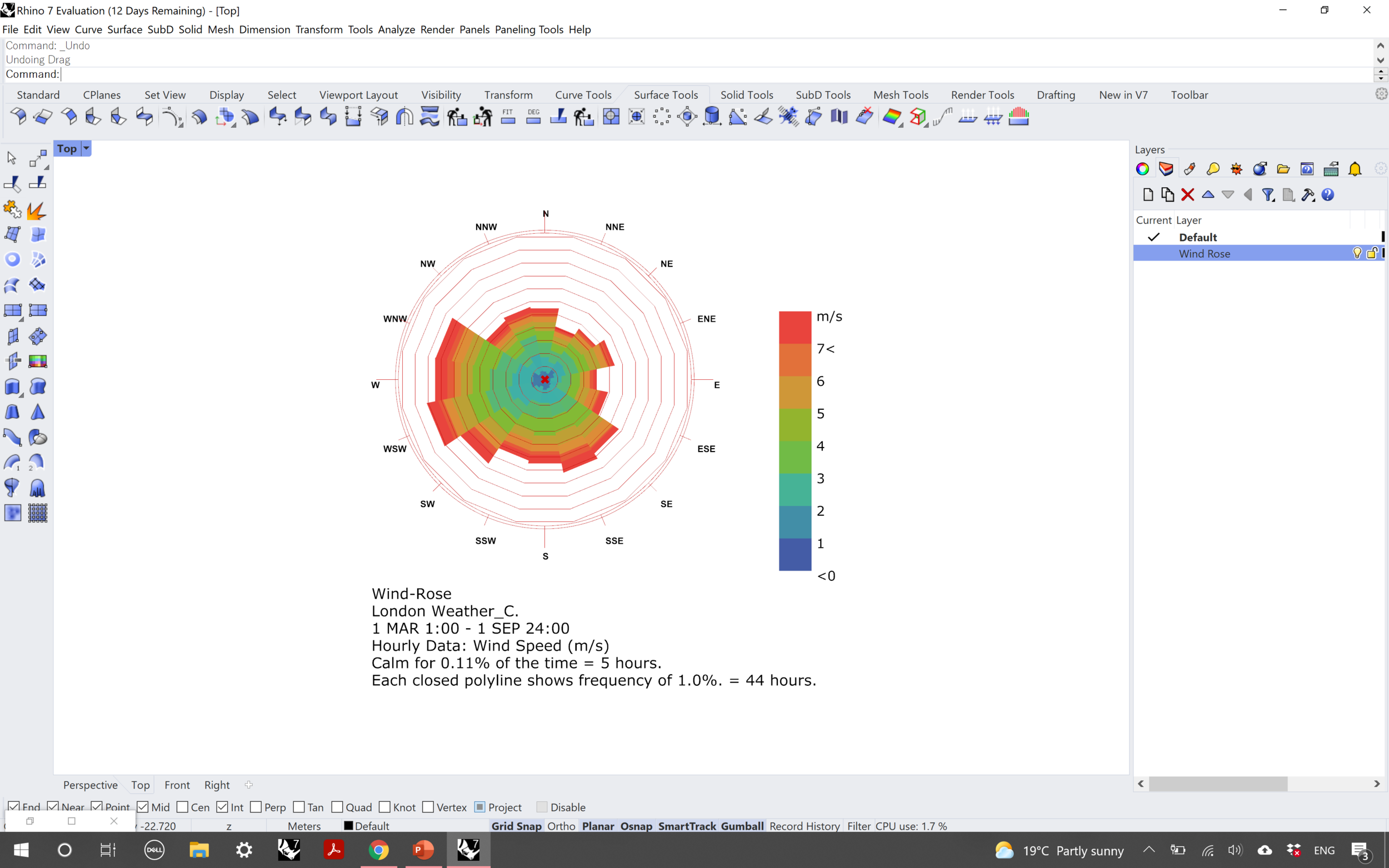
Once again, select the Rendered view style to finish off your windrose. You can now export this as an image file to use in your environmental analysis of your site.
This brings us to the end of a very long, but hopefully useful tutorial on some representations of environmental site analyses. Grasshopper can be daunting if you haven’t scripted anything before, but once you get to grips with a few of the features you’ll appreciate it as an additional tool to help you in your architectural projects.
Make sure to follow @archidabble on Instagram, and get in touch with us if you have any questions or blog post ideas you want to share with us!